Theory of Production and Cost – CA Foundation Economics Notes Chapter 3

Browsing through CA Foundation Business Economics Notes Chapter 3 Theory of Production and Cost help students to revise the complete subject quickly.

Theory of Production and Cost – Business Economics CA Foundation Notes Chapter 3

Meaning of production:
→ Production is one of the important economic activity that takes place in any economy apart from consumption and investments.

→ An individual firm is the micro-economic unit which undertake the production of goods and services.

→ A firm’s survival depends upon whether it is able to achieve optimum efficiency in production by minimizing the cost of production.

→ Production is the transformation of resources into goods and services. In other words, production is the act of transformation of Inputs into Output which satisfies the wants of some people. Example – Inputs of sugarcane, capital and labour are used to produce Sugar.

→ Production also includes production of Services like those of lawyers, teachers, doctors, etc.

→ The amount of goods and services that an economy is able to produce determines whether it is rich or poor. A country like U.S.A. is a rich country as its production level is high.

→ Man cannot create or destroy matter.

→ In Economics, the term production means creation of economic utilities in the matter i.e. in the things that already exist.

→ Thus, production means creation of those goods and services which have economic utilities i.e. exchange value.

→ According to James Bates and J.R. Parkinson, “Production is the organized activity of transforming resources into finished products in the form of goods and services; and the objective of production is to satisfy the demand of such transformed resources.”

→ Professor J. R. Hicks has defined production “as any activity whether physical or mental, which is directed to the satisfaction of other people’s wants through exchange.”

→ The definition indicates that the term production covers the whole process from creation of utilities till the satisfaction of human wants.

→ Utilities may be created or added in many ways, such as :
1. Form Utility:

• It is created by changing the form of raw materials into finished goods for man’s use.
• Example – converting raw cotton into cotton fabric.
• Form utility is created by manufacturing industries.

2. Place Utility:

• It is created by transporting goods from one place to another.
• Example – when goods are taken from factory to marketplace, place utility is created.
• Transport services are involved in creation of place utility.

3. Time Utility:

• It is created by making things available when they are required.
• Example – Banks create time utility by granting overdraft facilities.

4. Service Utility (Personal Utility):
It is created by providing personal services to the customers by professionals likes lawyers, doctors, bankers, shopkeepers, teachers, transporters, etc.

Factors of Production:

Land:
→ Generally, land means earth’s surface.

→ However, in economics land refers to all the free gifts of nature i.e. natural resources. Land includes natural resources:

• on the surface of earth; Example – Soil, forest, plots of land, etc.
• below the surface of earth, Example – mineral deposits, etc. and
• above the surface of earth, Example – climate, sunshine, rain, etc.

→ Land has the following characteristics:

• Primary Factor. Land is the original and primary or natural factor of production. It provides various natural resources for production.
• Free Gift of Nature. Land is the creation of nature and not man made. It is a free gift of nature to mankind.
• Inelastic Supply. Land is fixed in supply. Its supply cannot be either increased or decreased by any human efforts. However, its supply is relatively elastic from the point of view of a firm.
• Lacks Geographical Mobility. Land cannot be moved bodily from one place to another. However, land is said to be mobile in the sense it can be put to many alternative uses.
• Passive Factor. Land does not yield any result unless human efforts and capital are employed.
• Heterogeneous. Land differs in nature, fertility, uses and productivity from one place to another.
• Permanent. It means that land cannot be destroyed. The productive power of soil is original and indestructible according to Ricardo.
• Diminishing Returns. The land is subject to the Law of Diminishing Returns more quickly in the cultivation of land.

Labour:

• Labour in economics means any work whether physical or mental done in exchange for some monetary reward.
• Anything done out of love and affection is not labour in economic sense.
• Labour has the following peculiarities (characteristics) which makes it different from other factors:

1. Labour is inseparable from labourer:

• All other suppliers of factors can be separated from the factors which they supply.
• Example – Land can be separated from its owner.
• However, the labourer cannot be separated from the work which he performs.
• Example – A doctor has to attend his patients in person. Labour is connected with Human Efforts.

2. Human Factor:

• It is a live factor of production. Hence, labour has feelings and temperament.
• So it is very much affected by surroundings, working, conditions, motivation, leisure, recreation, working hours, etc.

3. Highly perishable:

• Labour cannot be stored for future use. It is highly perishable.
• A day lost without work means a day’s work gone forever.
• Hence, labourer has weak bargaining power and has to accept even low wages.

4. The labourer sells his services and not himself:
In the labour market it is labour which is brought and sold and not the labourer.

5. Heterogeneous:

• Labour power differs from labourer to labourer.
• Labour power depends upon physical strength, education, skill, training, efficiency,
• Hence, labour can be classified as unskilled, semi-skilled and skilled labour.
• The skilled labour is called as human capital.

6. Mobile.

• Labour is a mobile factor.
• Labour is much less mobile than capital.
• Labourer is human being and hence has attachment with his family, custom, religion, culture, etc. and so is hesitant to move from one place to another.

7. Active Factor:
Labour is the most active factor of production. Other factors are made operative with the use of labour.

8. Labour has sociological characteristics:

• Employment of labour involves problems relating to labour welfare.
• Example – Social security like provident fund, gratuity, medical benefits, pension, etc.
• Other factors do not have such characteristics.

9. Supply curve of labour is backward sloping.

10. The supply of labour is inelastic in short run.

Capital:
→ In ordinary language, capital is used in the sense of money.

→ But in economics the term ‘Capital’ means man made stock of goods like factories, machines, tools, equipments, raw materials, dams, canals, transport vehicles, etc. which are used in production.

→ Thus, ‘Capital’ in economics is used in the sens(e of real capital i.e. capital goods.

→ Capital has therefore, been rightly defined as “produced means of production” and as “man made instrument of production”.

→ Land and labour are primary or original factors of production. But capital is produced by man working with nature to help in the production of further goods.

Following are the main characteristics of capital:
1. Capital is man made:
Capital is not produced by nature. It is artificial as it is produced by man.

2. Capital is productive:
Use of capital increases the overall productivity in a given process. It provides tools and implements to labour for production.

3. Supply of capital is elastic:

• The supply of capital can be adjusted to demand.
• The stock of capital depends on capital formation.
• Thus, by raising the rates of savings and investments the supply of capital can be increased.

4. All capital is wealth:

• Capital is that part of wealth which is used in further production of wealth.
• Hence, capital has all the characteristics of wealth like utility, scarcity, transferability and price.

5. Capital is a passive factor:
It alone is unable to produce anything. It is ineffective without the use of labour and land.

6. Capital is the most mobile factor:
It has both place as well as occupational mobility.

7. Capital is durable:
Physical capital assets like plant and machinery, factory buildings, etc. last over a long time in the process of production. However, they are subject to depreciation.

8. Capital involves social cost:

• In the creation of capital, the money to be used for present consumption has to be diverted.
• Sacrifice of present consumption and enjoyment of the people is treated as a social cost.

Types of capital:

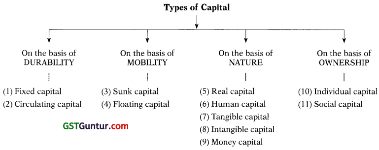
→ Fixed Capital. Those durable physical assets which can be repeatedly used in the process of production for long periods are called fixed capital.
Example – Machinery, Plant, Tools, Factories, Railways, etc.

→ Circulating or Working Capital. Working capital refers to those goods which are used up in the single act of production. Such goods are used only ONCE in production.
Example – raw materials, power, fuel, etc. They are single use producer’s goods.

→ Sunk Capital. Sunk capital is the capital which is used to produce only one single commodity. It can be put to a single specialized use only.
Example – A brick kiln can be used only to bake brick and nothing else. Sunk capital therefore, lacks occupational mobility.

→ Floating Capital. Floating capital is that which can be put to several uses.
Example – electricity, money, leather, etc.

→ Real Capital. Real capital refers to the physical capital goods like machinery, raw material, factory buildings, etc. which help in production.

→ Human Capital. The human capital is in the form of people who are equipped with education, skills, training, good health, etc. A faster economic growth can be achieved with the accumulation of human capital.

→ Tangible Capital. Tangible capital is one which can be seen and touched.
Example – machinery, tools, etc. in other words, it is real capital.

→ Intangible Capital. It cannot be seen or touched. It can only be felt.
Example – goodwill, etc.

→ Money Capital. It is in the form of shares, debentures, bonds, stock certificates, etc. Money is invested in expectations of returns.

→ Individual Capital. Capital resources having personal or private ownership of an individual or group of individuals is called individual capital.
Example – Tata Enterprises.

→ Social Capital. The capital which is owned by the society as a whole is called as social capital.
Example – roads, railways, schools, dams, canals, etc.

Capital Formation:

• Capital formation means a sustained increase in the stock of real capital in a country.
• It is thus, an addition of capital goods like machines, tools, factories, transport facilities, power, etc. in the country.
• Such capital goods are used for further production of goods and thus increases the production capacity of the country.
• Capital formation is also known as investment.
• Capital formation plays an important role in the development of an economy generally, higher the rate of
• capital formation, more economically developed an economy would be.

There are mainly three stages of capital formation which are as follows:
1. Savings:
→ Savings represents that part of income which is not consumed. Level of savings in a country depends on –

• ability to save
• willingness to save.

(i)

• Ability to save depends upon the income of an individual.
• Higher the income, higher is the savings.
• This is because with the increase in income the propensity to consume falls and propensity to save increases.
• This is true in case of both the individuals and the economy.

(ii)

• A person with ability to save must also have willingness to save.
• Willingness to save depends upon individual’s concern about future. If a person is foresighted and wants to make future secure, he will save more.
• Willingness to save also depends upon family affection, desire for the growth and promotion of business, desire for prestige and power habits, sound banking system, stability in the money value, State’s taxation policy, etc.

2. Mobilization of Savings:

• The money so saved by the households must enter into circulation i.e. must be mobilized and make them available to the businessmen or entrepreneurs who require it for investment purposes.
• This requires a network of banks, financial institutions (like UTI, IDBI, etc.), insurance companies, etc.
• Such facilities help to promote high rate of mobilization and canalization of savings.

3. Investments:

• The final stage is the investment of savings into capital assets like machinery, tools, buildings, dams, etc.
• Investment requires a large number of honest, dynamic, daring, efficient and skilled entrepreneurs in the economy.
• Investments also depends upon the factors like expected profits, rate of interest, size of market, stability in the money value, internal peace and security, fear of foreign aggression, etc.

Entrepreneur:

• The most important factor in production i.e. enterprise is provided by entrepreneur.
• An entrepreneur is a person or group of persons who bring together the different factors of production i.e. land, labour and capital at one place; combine them in right proportions; initiate the process of production by making them work together and bear the risks and uncertainty involved in it.
• He is therefore also called the organizer, the manager or risk bearer.

An entrepreneur performs the following functions:
1. Initiating a business enterprise:

• The first function of an entrepreneur is to start a business. For this he brings together the different factors of production like land, labour and capital.
• He pays them their respective remuneration i.e. rent for land, wages to labour and interest to capital.
• Any surplus left after factor payment is his reward i.e. profit which is not fixed.
• If his planning goes wrong he may also incur losses.

2. Risk and Uncertainty bearing:
→ Main function of an entrepreneur is to bear risk and uncertainty. According to Prof. F. H. Knight there are two types of risks namely –

• Foreseeable or insurable risks, example – risk of fire, thefts, accidents, etc.
• Unforeseeable or non-insurable risk, example – technological risks due to inventions, fluctuations in demand due to change in fashion etc., trade cycles, changes in govt, policies, etc.

→ Foreseeable risks can be predicted and hence can be insured. Such risks do not cause uncertainty and thus do not give rise to profits.

→ Unforeseeable risks involve uncertainty and give rise to profits.

→ True entrepreneurship lies in bearing non-insurable risks and uncertainties.

3. Innovations:

• Prof. Joseph A. Schumpeter considers innovation as the true function of the entrepreneur.
• Innovation refers to all those changes in the production process the objective of which is to reduce the cost of production and increase profits.
• Innovations in wider sense includes introduction of new or improved production methods, a new machine, a new plant, use of a new source of raw material, change in the internal organizational set-up, etc.
• Such innovations give rise to profits but temporarily because once these are adopted by other firms, the profits could disappear.
• Hence, entrepreneur has to continuously introduce new innovations and contribute to technological progress and economic growth of the country.

Enterprise’s objectives and constraints:
→ Earning profit is considered to be the prime objective of every business. However, earning profit cannot be the only objective of the business because an enterprise functions in the economic, social, political and cultural environment. Hence, an enterprise has to set us objectives in relation to such environment. The objectives of an enterprise are as follows:
(1) Organic objectives: The basic purpose of all kinds of enterprises is to Survive and Exist i.e. to stay alive. This is possible only when it is able to recover its costs and earn profits. Once the enterprise is assured of its survival, it will aim at growth and expansion.

• Growth as on objective has gained importance with the rise of professional managers. H.L. Marris’s and other economists assert that managers of a corporate firm are interested in maximizing the growth rate rather than in profit maximization.
• Owners are interested in profits, capital, market share and public reputation.
• For growth and expansion of the firm it is necessary that adequate profits are made so as to provide internal funds for further investment.
• Growth and profit are both positively related to the size of the firm. Both of the objectives converge in one namely A Steady growth in the size of the firm.
• Managers prefer balanced rate of growth over profits. The growth rate and growth is measured in terms of sales, number of branches, number of employees, etc.

(2) Economic Objectives: The basic and important objective of every business is to earn profit. Accordingly therefore, the firm determines the price and output policy in a manner that profits can be maximized.

• Investors expect sufficient returns from their company. Similarly, creditors and employees are also interested in profitable enterprise.
• The definition of profits in economic sense has different meaning than accountants definition of profits.
• Accounting Profit = Total Revenue – Accounting Cost (Explicit Cost)
• Economic Profit = Total Revenue – Economic Cost (i.e. Explicit + Implicit Cost)
• Profit maximization objective has been criticized because all firms do not aim to maximize profits.

Example :

• Some firm try to achieve Security with reasonable level of profit.
• Some firms may try to Maximise Sales (Prof. Baumol)
• Some economists point that owners and managers of a company try to Maximise their utility rather than profit.

(3) Social Objectives: A business enterprise is an integral part of society. It lives in a society. It cannot grow unless it meets the needs of the society. It makes use of resources of j society. Therefore, it owes something to society. Some of the important social objectives j of business are –

• To maintain continuous and desired quantity of unadulterated goods of standard quality.
• To avoid unfair trade practices.
• To avoid profiteering and anti-social practices.
• To create opportunities for gainful employment for the people in the society. A business should specially consider the handicapped, disabled and poor people.
• To avoid air, water or noise pollution.

(4) Human Objectives: Employees are precious resources who contribute abundantly to the success in business. Therefore, the overall development of its employees, keep them motivated and taking care of employees should be major objectives of an organization.

The common human objectives are –

• To provide fair deal to the employees at different levels.
• To provide good working conditions.
• To pay competitive and satisfactory wages and salaries.
• To impart training to employees and keep updating their knowledge.
• To provide opportunities to employees in decision making process on the matters affecting them.

(5) National Objectives: An enterprise should try to fulfil the nations need and aspirations. It should work towards implementation of national plans and policies. Some of the national objectives are –

• To remove inequality of opportunities and provide opportunities to all irrespective of caste and religion to work and to progress.
• To produce according to national priorities.
• To help country achieve self-sufficiency in production of all types of goods and thus reduce dependence on other countries.
• To provide education and training to young men to bring about skill formation for achieving growth and development.
• All the enterprises have multiple objectives and therefore, the need to set priorities by balancing of the objectives.

In the pursuit of the above objectives an enterprise’s action may get constrained in following ways –

• Lack of knowledge and information about many variable that affect business.
• Constraints may be experienced due to governments’ restrictions on the production, price and movement of factors.
• There may be infrastructural bottleneck.
• Changes in business and economic conditions; change in government policies about location, prices, taxes, etc.; natural calamities like fire, flood, famine, etc.
• Constraints are also faced due to inflation, rising interest rates, unfavourable exchange rate, capital and labour costs, etc.

Enterprise’s Problems
→ A business enterprise face many problem from its start, through its life time till it is closed down. Following are the main problems:
(1) Problems relating to objectives: An enterprise functions in the economic, social, political
and cultural environment. Therefore, it has a set of many objectives in relation to its environment.

• These multifarious objectives many times conflict with one another. Hence, the enterprise faces the problem of choosing and striking balance between them.
• Example – Social responsibility objective may run into conflict with expansion of production activity resulting in pollution.

(2) Problems relating to location and size of the plant: An enterprise has to decide about the Location of its plant. In doing so, it has to consider many costs like cost of labour, facilities and cost of transportation to decide where its plant should be located.

→ Another problem faced is about SIZE of the firm, whether it should be a small scale or large scale unit. Before deciding upon the scale of operations several aspects will have to be considered like technical, managerial, marketing, financial, etc.

(3) Problems relating to selecting and Organising physical facilities: A firm has to decide about the nature of production process to be used and the type of equipments required for it. This will depend upon the require volume of production
→ This choice will be based on –

• the evaluation of costs of different equipments
• efficiency

→ It has also to prepare layout of plant.

(4) Problems relating to Finance: A firm also has to do good financial planning. For this an enterprise will have to determine –

• amount of funds required
• demand and cost of its products
• profits on investments, and
• capital structure

(5) Problems relating to Organisation Structure: An enterprise faces problem relating to organizational structure. It has to divide the total work of the enterprise by creating different departments in order to carry on the specialized functions by each department.

• It has to clearly define the roles and relationships of all positions also.

(6) Problems relating to Marketing: For survival and growth, a firm has to properly do marketing of its products and services.

• It has to identify its actual and potential customers, tools of marketing, etc.
• After identifying the market, the firm has to decide upon product, promotion, price and place aspects.

(7) Problems relating to Legal Formalities: Many legal formalities are to be carried out at the time of formation, during the life time and at closure.
Example – assessing various taxes and paying, maintenance of records, filing various returns, adhering to laws formulated by Govt., etc.

(8) Problems relating to Industrial Relations: This problem relates to winning worker’s co-operation, enforcing discipline among workers, workers participation in management, dealing with trade unions, etc.

Production Function:
→ Output is a function of inputs i.e. factor services such as land, labour and capital which are used in production. In other words, production is a transformation of Physical Inputs into Physical Output.

→ The functional relationship between physical inputs and physical output, per unit of time under a given state of technology is called production function.

→ It can also be expressed in the form of a mathematical equation in which output is the dependent variable and inputs are the independent variables.
Q = f (a, b, c …………. n)
Where –
Q denotes quantity of output of a commodity per unit of time
f stands for function of i.e. depends on a, b, c,… n denotes quantity of various inputs.

Assumptions of Production Function:
The production function is based on the following assumptions:

• It is specified with reference to a specified period of time.
• It is assumed that the state of technology remains the same, during the period of time.
• It is assumed that the firm uses best and most efficient technique available in production.
• It is assumed that the factors of production are divisible into viable units.

The production function can be explained under two heads:
1. The short run production function in which input – output relations are analysed where –

• One input is variable, all other inputs are fixed, (described as the Law of Variable Proportions) OR
• Two inputs are variable, all other factors are fixed (explained with the help of isoquants)

2. The long run production function in which input- output relations are analysed where all the inputs are variable (described as the Law of Returns to Scale).
Cobb-Douglas Production Function:
Q = f (L, K). Where –
Q = Output; L = Labour; K = Capital

→ Paul H. Douglas and C.W. Cobb of the U.S.A. studied the production function of the American manufacturing industries. This production function applies to the whole of manufacturing in U.S.A. rather than to an individual firm. In this case, output is manufacturing production and inputs used are labour and capital.

→ The conclusion of study is that labour contributed 3 /4th and capital about 1 /4th in the manufacturing production.

Fixed Inputs (Fixed Factors) and Variable Inputs (Variable Factors):

Comparison	Fixed Inputs	Variable Inputs
(i) Meaning	1. The factors which cannot be easily and quickly changed and require long time to make adjustment in them with the changes in the level of output are called fixed inputs or fixed factors of production. 2. In other words, factor inputs whose quantity does not vary from day-to-day are called as fixed inputs.	1. The factors which can be easily and quickly changed and readily adjusted with the changes in the level of output are called variable inputs or variable factors of production. 2. In other words, factor inputs whose quantity may vary from day-to-day are called as variable inputs.
(ii) Examples	1. Examples of fixed inputs – buildings, machinery, plant, top management, etc. 2. It requires long time to make variations in them. 3. Example – To construct a new factory building with a larger area and capacity.	1. Examples of variable inputs – ordinary labour, raw-material, power, fuel chemicals, etc. 2. It can be readily changed.
(iii) Relation with Output	1. Fixed inputs do not vary with the level of output. 2. Its quantity remains the same, whether the output is more or less or zero in Short run.	1. Variable inputs vary directly with the level of output. 2. Such factors are required more, when output is more; less, when output is less and zero, when output is zero in Short run.
(iv) Cost	1. The cost of the fixed inputs is called Fixed cost. 2. In the short run the firm has to bear the fixed cost even if the output is zero. 3. Since the quantity of fixed inputs remains the same, fixed cost remains the same whatever be the level of output.	1. The cost of the variable inputs is called Variable cost. 2. Since variable inputs vary directly with the level of output, variable costs are also positively related with output. If output is zero, variable cost is also zero. 3. If output is increased variable cost also increases and vice-versa.

Short Run (Short Period) & Long Run (Long Period):

Comparison	Short Run	Long Run
(i) Meaning	1. The short run is defined as the period of time in which some factors of production or at least one factor is fixed i.e. does not vary with output 2. Thus, in the short period some factors are Fixed Factors → Example – Factory building, machinery, management, etc. and some are Variable factors. → Example – Labour, raw-material, power, fuel, etc..	1. The long run is defined as the period of time in which all factors may vary. 2. In the long run, all factors become variable and so there is no distinction between fixed and variable factors.
(ii) Scale of Production OR Size of the Firm	1. In the short run, the output is produced with a Given scale of production i.e. the size of plant or firm (and so the production capacity) remains unchanged. 2. Hence, production can be increased or decreased only by changing the amount of variable factors	1. In the long run, the output is produced with the Change in the scale of production i.e. the size of plant or firm can be increased (and so the production capacity). 2. Hence, production can be increased by varying all factors i.e. fixed factors (of short period) as well as variable factors.
(iii) Production Law	The production function which is studied in the short run period is called as the Law of Variable Proportions.	The production function which is studied in the long run period is called as the Law of Returns to Scale.
(iv) Decisions about Change in factors	1. The decisions to change the amount of variable factors (like raw material, labour, etc.) are taken very frequently depending upon changes in demand of the commodity. 2. Hence, short run is the ‘Actual production period’ during which some factors are fixed while some are variable. 3. Thus, firms operate in the short run period.	1. The decisions to change the amount of fixed factors i.e. scale of production or to close down the firm are taken only once in a while. 2. Hence, long run is the ‘Planning period’. 3. Thus, firms plan in the long run period.
(v) Nature of Supply	1. In the short run period, supply can be adjusted up to a limited extent as per changes in demand. 2. In other words, supply is relatively inelastic.	1. In the long run period, supply can be fully adjusted as per changes in demand. 2. In other words, supply is relatively elastic.
(vi) Nature of Cost	1. In short run period, cost is classified as Fixed Cost and Variable Cost. 2. Fixed cost is the cost of fixed inputs and Variable cost is the cost of variable inputs. 3. Fixed cost is the main feature of short run period	1. In long run period All costs are variable. 2. Variable cost is the main feature of long run period.
(vii) Effect on Price	1. In short-run, the price determination of a commodity is more influenced by – → The demand forces than supply forces because supply in short-run is relatively inelastic. → The UTILITY of the commodity.2. The short-run price is called Sub-Normal Price	1. In long-run, the price determination of a commodity is more influenced by – → The supply forces than demand forces because supply in long-run is relatively elastic. →  The Cost of Production of the commodity.2. The long-run price is called Normal Price.
(viii) Average Cost Curve	1. The short-run average cost curve is ‘U’ shaped. 2. Its U-shape is explained with the Law of Variable Proportions.	1. The long-run average cost curve is also U shaped. 2. But its U- shape is not as prominent as short-run average cost curve. 3. Its U-shape is explained with the Law of Returns to Scale. 4. Long-run average cost curve is also called ‘Planning Curve’ and ‘Envelope Curve’.
(ix) Profit of Firms	In the short-run period – (a) The firms under perfect competition on being at equilibrium may earn normal profits, super normal profits or incur losses. (b) The monopoly firm on being at equilibrium may earn normal profits, super normal profits or incur losses. (c) The firms under monopolistic competition on being at equilibrium may earn normal profits, super normal profits or incur losses.	In the long run period – (a) The firms under perfect competition earn only Normal profits and operate at optimum level. (b) The monopoly firm can earn Super Normal profits and operate at sub-optimum level. (c) The firms under monopolistic competition earn only Normal Profits and operate at sub-optimum level.

Concepts of Product:
→ Product i.e. output refers to the volume of goods produced by a firm in a particular period of time.

→ There are three concepts relating to the physical production by factors namely –

• Total Product (TP),
• Average Product (AP), and
• Marginal Product (MP).

1. Total Product (TP).

• The total output produced by all the factors per unit of time is called total product.
• Total product increases with an increase in the variable factor input.
• Column Nos. (1) and (2) of the following table shows a total product schedule.

2. Average Product (AP):
→ The. average product means the total product per unit of a variable factor.

→ In other words, it is the total product divided by the number of units of a variable factor.
Average Product = \(\frac { Total Product }{ No.of units of Variable factor }\)
OR AP = \(\frac { TP }{ QVF }\)

→ Column No. (3) of the following table shows the average product of variable factor.

3. Marginal Product (MP):
→ The marginal product means addition made to total product by the use of an extra unit of variable factor.

→ It may be stated as –
MP = TP_n – TP_n-1
where,
MPn = Marginal product when ‘n ’ units of variable factors are used
TP = Total Product
n = number of units of variable factors used.

→ Marginal Product may also be defined as the change in total output due to use of additional unit of variable factor
MP = \(\frac { ∆ TP}{ ∆ QVF }\)
Where –
∆ = a small change Column No. (4) of the following table shows the marginal product schedule.
Table: Product Schedule

Units of Variable factor Example – Labour	Total Product(TP)	Average Product(AP)	Marginal Product(MP)
1	10	10	10
2	30	15	20
3	60	20	30
4	80	20	20
5	90	18	10
6	90	15	0
7	85	12.1	-5

→ Average product and Marginal product are related to one another.
(i)

• When average product of the variable factor is rising, marginal product of the variable factor is more than its average product.
• So when average product curve is rising, the marginal product curve will lie somewhere above it.

(ii)

• When average product of the variable factor is falling, marginal product of the variable factor is less than its average product.
• So when average product curve is falling, the marginal product curve will lie somewhere below it.

(iii)

• When average product of the variable factor is maximum and constant, marginal product is equal to average product.
• In other words, the marginal product curve cuts the average product curve at its maximum point.

Law of Variable Proportions:
→ The Law of Variable Proportions examines the production function i.e. the input-output relation in short run where one factor is variable and other factors of production are fixed.

→ In other words, it examines production function when the output is increased by varying the quantity of one input.

→ Thus, the law examines the effect of change in the proportions between fixed and variable factor inputs on output in three stages viz. Increasing returns, diminishing returns and negative returns.

→ Statement of the Law :
“As the proportion of one factor in a combination of factors is increased, after a point first the marginal and then the average product of that factor will diminish”. (F. Benhan)

→ The law operates under some assumptions which are as follows:

• There is only one factor which is variable. All other factors remain constant.
• All units of variable factor are homogeneous
• It is possible to change the proportions in which the various factors are combined.
• The state of technology is given and is constant.

The three stages of the law can be explained with the help of the following schedule and diagram.
Table : Law of variable proportions

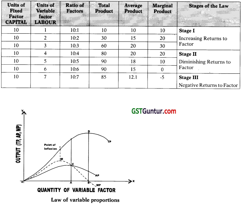
Stage I : The Law of Increasing Returns to Factor –

• During this stage, total product (TP) increases at an increasing rate upto the point of inflexion ‘I’ and thereafter it increases at diminishing rate.
• This is because marginal product (MP) of the variable factor increases upto point ‘M’ on MP curve and then start falling.
• Rising MP also pulls up average product (AP), which goes on rising, in the first stage.
• Rising AP indicates increase in the efficiency of variable factor i.e. labour.
• Stage I ends where AP is maximum and is equal to MP as shown by point ‘C’ in the diagram.

The law of increasing returns operates because of the following two reasons:
1. Indivisibility of fixed factors –

• Due to indivisibility, the quantity of fixed factors is more than the quantity of variable factors.
• So when the quantity of variable factors is increased to work with fixed factors, output increases speedily due to full and effective utilisation of fixed factors.
• In other words, efficiency of fixed factors increases.

2. Efficiency of Variable Factor Increases –
Due to increase in the quantity of variable factor, it becomes possible to introduce Divison of Labour leading to Specialistion. This results in more output per worker.

Stage II : The Law of Diminishing Returns to Factor –

• In second stage, TP continues to increase at diminishing rate. It reaches the maximum at point ‘D’ in the diagram, where the second stage ends.
• In this stage, both AP and MP of variable factor are falling- though remains positive. That is why this stage is called as the stage of diminishing returns.
• At the end of this stage MP becomes, zero as shown by point ‘B’ in the diagram and corresponding to highest point ‘D’ on TP curve.

The law of diminishing returns operate due to the following two reasons:
1. Indivisibility of fixed factors –

• Once the optimum proportion between indivisible fixed factors and variable factors is reached (as in Stage I) with any further increase in the quantity of Variable factor, the fixed factors become inadequate and are overutilised.
• The fine balance between fixed and variable factor gets disturbed. This causes AP and MP to diminish.

2. Imperfect Substitutability of factors:

• Variable factors are not perfect substitute of fixed factors.
• The elasticity of substitution between factors is not infinite.

Stage III : The Law of Negative Returns to Factor –

• In third stage, TP falls and so, TP curve slopes downward. MP becomes negative and the MP curve goes below the X-axis. AP continues to fall.
• As the MP of variable factor becomes negative, this stage is called the stage of negative returns.
• In this stage the efficiency of fixed and variable factors fall and factor ratio becomes highly sub-optimal.

The law of negative returns operate due to the following reasons:

• The quantity of the variable factor becomes too excessive compared to fixed factors. They get in each other’s way and so TP falls and MP becomes negative.
• Too large number of variable factors also reduce the efficiency of fixed factors.

Conclusion -Where to operate?

• A rational firm will not produce either in Stage I or in Stage III.
• In stage I, the marginal product of fixed factor is negative as its quantity is more than variable factor.
• In stage III, the marginal product of variable factor is negative as its quantity is too large than fixed factor.
• Therefore, firm would seek to produce in Stage II where both AP and MP of Variable factor are falling.
• At which point to produce in this stage will depend on the prices of factor inputs.

Law of Returns to Scale:
→ The Law of Returns to Scale examines the production function i.e. the input – output relation in long run where increase in output can be achieved by varying the units of All factors in the same proportion.

→ Thus, in long run all factors become variable.

→ It means that in long run the scale of production and the size of the firm can be increased.

→ The law of returns to scale analyse the effects of scale on the level of output as –
1. Increasing Returns to Scale:

• When the output increases by a greater proportion than the proportion increases in all the factor inputs, it is increasing returns to scale.
• Example – When all inputs are increased by 10% and output rises by 30%.
• The reasons of increasing returns to scale are – internal and external economies of scale; indivisibility of fixed factors; improved organisation; division of labour and specialisation; better supervision and control; adequate supply of productive factors, etc.

2. Constant Returns to Scale:

• When the output increases exactly in the same proportion as that of increase in all factor inputs, it is constant returns to scale.
• Example – When all inputs are increased by 10% and output also rises by 10%.
• The reason of constant returns to scale is that beyond a certain point, internal and external economies are Neutralised by growing internal and external diseconomies.

3. Diminishing Returns to Scale:

• When the output increases by a lesser proportion than the proportion increase in all the factor inputs, it is diminishing returns to scale.
• Example – When all inputs are increased by 20% but output rises by 10%.
• The reason of diminishing returns to scale is increased internal and external diseconomies of production.
• Internal diseconomies like difficulties in management, lack of supervision and control, delay in decision-making etc.
• External diseconomies like insufficient transport system, high freights, high prices of raw materials, power cuts, etc.

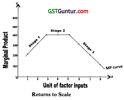
→ The law of returns to scale can also be illustrated with the help of the following schedule and diagram.
Table : Law of returns to scale

Units of Labour & Capital	Marginal Product (Units)	Total Product (Units)	Remarks
1 2	200 300	200 500	Stage I Increasing Returns
3 4 5	400 400 400	900 1300 1700	Stage II Constant Returns
6 7 8	300 200 100	2000 2200 2300	Stage III Diminishing Returns.

Returns to Factor and Returns to Scale:

	Returns to Factor	Returns to Scale
1. Meaning	1. Returns to factor refers to the various production sizes where one factor is variable and other factor of production are fixed. 2. In other words, it examines production function when the output is increased by varying the quantity of one input. 3. It examines the effect of Change in the proportions between inputs on output.	1. Returns to scale refers to the various production sizes where increase in output can be achieved by varying the units of All Factors in the Same Proportions. 2. It show the effects on output when all factor inputs are varied in the same proportion simultaneously.
2. Nature of Inputs	1. Quantities of some inputs are fixed while the quantities of other inputs vary. 2. In other words, there are Fixed and Variable factors of production.	1. Quantities of all inputs can be varied. 2. In other words, all factors of production are Variable.
3. Time Element	Returns to factor is called a Short Run production function.	Returns to scale is called a Long run production function.
4. Application	It does not apply where the factors must be used in fixed proportion to produce a commodity.	It does apply where the factors must be used in fixed proportions to produce a commodity.
5. Stages of Law	1. The law has three stages namely – Increasing Returns to factor, Diminishing Returns to Factor, & Negative Returns to factor 2. Of the three stages, diminishing returns pre-dominate.	1. The law has three stages namely – Increasing Returns to Scale, Constant Returns to Scale, Diminishing Returns to Scale. 2. All the three stages of return appear.
6. Causes of Operation	1. Increasing returns to factor is due to indivisibility of fixed factors and division of labour and specialisation. 2. Diminishing returns is due to non- optimal factor proportion and imperfect substitutability of factors. 3. Negative returns fall in the efficiency of fixed and variable factors.	1. Increasing returns to scale is due to increased internal and external economies. 2. Constant returns to scale is due to the fact that internal and external economies are neutralised by growing internal and external diseconomies. 3. Diminishing returns is due to internal and external diseconomies of scale.
7. Scale of Production	1. The scale of output is unchanged and the production plant or the size and efficiency of the firm remain constant. 2. This is because, only one factor is variable and all other factors are fixed.	1. The scale of output can be increased and so the size of the firm too can be expanded. 2. This is because all factors are variable and hence can be increased in the same proportion simultaneously.

Production Optimisation:

Isoquants:
An iso-product curve or isoquant is a curve, which represents the various combinations of two variable inputs that give the same level of output. As all combinations on the iso-product curve give the same level of output, the producer becomes indifferent to these combinations. That is why iso-product curve are also called ‘production indifference curve’ or ‘equal product curve’. To understand consider the following production isoquant schedule.

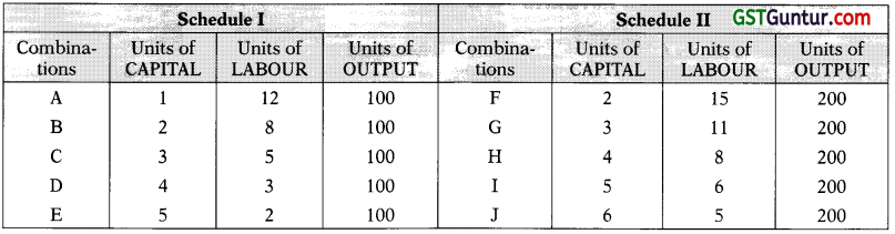
In the schedule I above, the producer is indifferent whether he gets combination A, B, C, D or E. This is because all the combinations of capital and labour give the same level of output i.e. 100 units.

By plotting the above combinations on a graph, we can derive an iso-product curve as shown in the following figure:

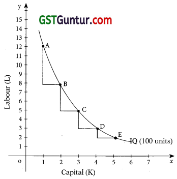
In the diagram, quantity of capital is measured on X-axis and quantity of labour on Y-axis.

The various combinations A, B, C, D, E of capital and labour are plotted and on joining them we derive an iso-product curve. All combinations lying on the iso-product curve yield the same level of output i.e. 100 units and hence technically equally efficient.

If the production schedule II is also plotted on the graph, we will get another iso-product curve IQ₂₀₀. This will lie above the IQloo as the combinations contain greater quantities of capital and labour. A set of iso-product curves is called iso-product curve map.

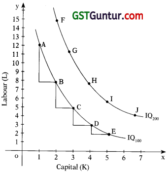
In the diagram, it can be observed that each iso-product curve is labelled in terms of output. All combinations lying of IQ₁₀₀ give the output of 100 units and all the combinations lying on IQ₁₀₀ give the output of 200 units. Higher iso-product curve represent higher level of output. Also it indicates how much more output can be achieved.

Marginal Rate of Technical Substitution:
The rate at which one factor of production is substituted in place of the other factor without any change in the level of output is called as the marginal rate of technical substitution. Consider the following schedule.

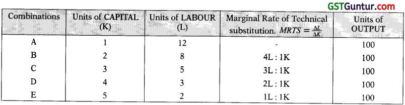
Each of the factor combinations in the table above yields same level of output. Moving from com-bination A to B, one unit of capital replaces 4 units of labour. Similarly, moving from B to C, one unit of capital now replaces only 3 units of labour and so on. It implies that labour and capital are imperfect substitutes. That is why MRTSKL is continuously diminishing. We can measure MRTSKL on an iso-product curve.

‘Iso-Cost Line’ OR ‘Equal Cost Lines’:
Iso-cost line (also known Equal Cost Line; Price Line; Outlay Line; Factor Price Line) shows the various combinations of two factor inputs which the firm can purchase with a given outlay (i.e. budget) and at given prices of two inputs.

Example:
A firm has with itself ₹ 1,000 which it would like to spend on factor ‘X’ and factor ‘Y’.
Price of factor ‘X’ is ₹ 20 per unit.
Price of factor ‘Y’ is ₹ 10 per unit.
Therefore, if the firm spends the whole amount on factor X, it can buy 50 units of X and if the whole amount is spent on factor Y, it can buy 100 units of Y. However, in between these two extreme limits, it can have many combinations of X and Y for the outlay of ₹ 1,000. Graphically it can be shown as follows –

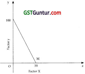
In the diagram OP shows 100 units of Y and OM shows 50 units of X. When we join the two points P and M, we get the iso-cost line. All the combinations of factor X and factor Y lying on iso-cost line can be purchased by the firm with an outlay of ₹ 1,000. If the firm increases the outlay to ₹ 2,000, the iso-cost line shifts to the right, if prices of two factors remains unchanged. The slope of the iso-cost line is equal to the ratio of the prices of two factors. Thus,
Slope of line PM = \(\frac { Price if X }{ Price of Y }\)

Producer’s Equilibrium OR Production Optimization:
A firm always try to produce a given level of output at minimum cost. For this it has to use that combination of inputs which minimizes the cost of production. This ensures maximization of profits and produce a given level of output with least cost combination of inputs. The least-cost combination of inputs or factors is called producer’s equilibrium or production optimization. This is determined with the help of (a) isoquants, & (b) iso-cost line.

An isoquant or iso-product curve is a curve which shows the various combinations of two inputs that produce same level of output. The isoquants are negatively sloped and convex to origin. The slope of isoquants shows the marginal rate of technical substitution which diminishes. Thus, MRTS_xy

Iso-cost line shows the various combination of two factor inputs which the firm can purchase with a given outlay and at given prices of inputs. There can be different outlays and hence different iso-cost lines. Slope of iso-cost line shows the ratio of the price of two inputs i.e. \(\frac{P_{x}}{P_{y}}\)

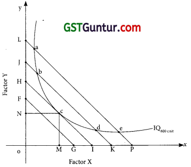
Which will be the least cost combination can be understood with the help of following figure. Suppose firm wants to produce 300 units of a commodity. It will first see the isoquant that represents 300 units.

In the adjoining diagram we find that all combinations a, b, c, d and e can produce 300 units of output. In order to produce 300 units firm with try to find out least cost combination. For this it will super impose the various iso-cost lines on isoquant as shown in the diagram.

The diagram shows that combination ‘C’ is,the least cost combination as here isoquant is tangent to iso-cost line HI. All other combinations a, b, d and e lying on isoquant cost more as these points lie on higher iso-cost lines. Hence, the point of tangency of isoquant and iso-cost line shows least cost combination. At the point of tangency.

Slope of iso-quant = Slope of iso-cost line
∴ MRTS_xy = \(\frac{P_{x}}{P_{y}}\)
Thus, the firm will choose OM units of factor X and ON units of factor Y and be at equilibrium as the marginal physical products of two factors are proportional to the factor prices.

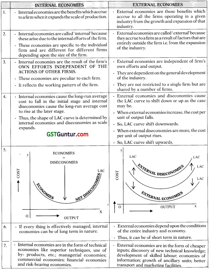
Internal Economies and Diseconomies:
→ Internal economies are those benefits which accrue to a firm when it expands the scale of production.

→ Internal economies are the result of the firm’s own efforts independent of the actions of other firms.

→ These economies are particular to the individual firms and are different for different firms depending upon the size of the firm.
The main types of internal economies are as follows –
1. Technical Economies:

• The large scale production is associated with technical economies.
• As the firm increases its scale of production, it becomes possible to use better plant, machinery, equipment and techniques of production.
• Following are the main forms (causes/reasons) of technical economies

Economies of superior techniques:

• A large sized firm can use sophisticated and costly machines and equipments.
• Use of superior techniques reduces the cost of production per unit and increases aggregate output.

Economies of increased dimensions:

• A large firm can get the mechanical advantage in using large machines and other mechanical units to produce more output.
• Example – A Large boiler, large furnace, etc. can be operated by same team as required by smaller boiler, furnace, etc.

Economies of linked processes:
A large sized firm can develop its own sources of raw material, means of transportation, distribution system, etc.

Economies of the use of By-products:

• A large sized firm can avoid all kinds of wastage of materials. The firm can use its by- products and waste material to produce another material.
• Example – Sugar industry can make alcohol out of the molasses.

Economies of specialization:
A large sized firm can introduce greater degree of division of labour and specialisation.

2. Managerial Economies:

• Large sized firms can introduce division of labour in managerial tasks.
• They can employ business executive of high skill and qualification to look after the functioning of various departments like production, finance, sales, advertising, personnel, etc.
• This helps to increase the efficiency and productivity of managers resulting in reduction in managerial costs.

3. Commercial Economies:

• A large sized firm is able to reap economies of bulk purchases.
• It can get discounts from suppliers, railways, transport companies, etc.
• It enjoys prompt and regular supply of raw materials.
• A large sized firm can also afford to spend large amount of money on advertising, publicity, etc.
• It can also give various concessions to wholesale and retail dealers and customers and thus capture markets for its product.

4. Financial Economies:

• A big firm enjoys goodwill among lenders or investors.
• For raising finance it can either borrow from bank as it can offer better security or it can raise finance by issuing shares, debentures and by inviting public deposits. Such opportunities are not available to small firms.

5. Risk Bearing Economies :

• A large firm is better placed to face the uncertainties and risks of business.
• A big firm producing many variety of goods is in a better position to withstand economic ups and downs. Therefore, it enjoys economies of risk bearing.

→ Internal diseconomies means all those factors which raise the cost of production per unit of a particular firm when the scale of production is expanded beyond the point of optimal capacity.

→ Such diseconomies of scale are as follows:
1. Production Diseconomies :

• Production diseconomies sets in when expansion of firm’s production beyond optimum size leads to rise in the cost per unit of output.
• Example – Use of inferior or less efficient factors due to non-availability of efficient factors raises the per unit cost of output.

2. Managerial Diseconomies:

• As the scale of production increases burden on management also increases.
• Co-ordination of work among different departments becomes difficult. Supervision and control over the activities of subordinates becomes difficult, decision taking is delayed, etc.
• As a result, wastage increase and the efficiency and productivity decrease.
• Per unit cost starts rising.

3. Technical Diseconomies :

• Every equipment has an optimum point at which it works more efficiently and economically.
• Beyond optimum point they are overworked and may result in breakdowns, heavy cost of maintenance, etc.

4. Financial Diseconomies:

• Expansion of production beyond the optimum scale results in increase in the cost of capital.
• It may be due to increased dependence on external finances.

5. Marketing Diseconomies:

• Selling diseconomies set in if the scale of production is expanded beyond optimum level.
• The advertisement expenditure and marketing overheads increase more proportionately with the scale.

External Economies and Diseconomies:
→ External economies are those benefits which accrue to all the firms operating in a given industry from the growth and expansion of that industry.

→ External economies are not related to an individual firm’s own cost reduction efforts.

→ These are common to all the firms in an industry and shared by many firms or industries.

→ The main types of external economies are as follows –
1. Technological Economies:

• When the whole industry expands, it may result in the discovery of new technical knowledge, firms pool manpower and finance for research and development resulting in new and improved methods of production and new inventions.
• Use of improved and better machinery improves production function and cost of production per unit falls.

2. Economies of Localization :

• When in an area, many firms producing the same commodity are set up, it is called localization of an industry.
• Due to localization there is expansion of railways, post & telegraph, banking services, insurance, setting up of booking offices by transport, companies, setting up of powerful transformer by electricity department, etc.
• All the firms get these facilities at low prices.

3. Economies of Information :

• As pointed earlier, firms pool their resources for research and development.
• All firms get the benefit of the research in terms of market information, technical information, information about governments economic policies, information about availability of new source of raw material, etc.
• Also, specialized journals give information about latest developments.

4. Cheaper Inputs:

• When an industry expands its needs for raw materials, machines, etc. also expand.
• This may result in exploration of new and cheaper sources of raw materials, machinery, etc.
• Also, the industries producing such inputs also expand in scale.
• Therefore, they can supply these inputs at lower prices.
• As a result the cost of production per unit of the firm using these inputs falls.

5. Growth of Ancillary Industries :

• With the growth of an industry, many firms specialized in the production of inputs like raw material, tools, machinery, etc. come up.
• Such firms are called ancillary units which provides inputs at lower cost to the main industry.
• Likewise, some firms may get developed by processing the waste products of the industry.
• Thus, wastes are converted into by-products. This reduces the cost of production in general.

6. Development of Skilled Labour:

• When an industry expands specialized institutions like colleges, training centers, management institutes, etc. develop.
• This results in continuous availability of skilled labour like technicians, engineers, management experts, etc.

7. Better transportation & Marketing Facilities :

• When an industry expands many specialized transporters also develop.
• The firm in need of specialized transport service can get them easily at cheaper rates.
• Also many new marketing outlets and specialized marketing institutions develop. The firm need not spend on developing its own marketing outlets.
• This reduces the cost.

→ The growth and expansion of an industry in a particular area beyond optimum level results in many disadvantages for firms in the industry.

→ Such disadvantages increases the costs of production of each firm.

→ Therefore, they are called external diseconomies. Some of the external diseconomies are as follows:
1. Diseconomies of Scarcity of Inputs :

• When an industry expands its need for raw materials, machines, tools and equipments, etc. also expands.
  Some inputs are such which cannot be totally substituted.
• The firms supplying these inputs come under pressure and may supply inputs at a higher price.
• This raises the cost of production per unit of the firm who uses these inputs.

2. Diseconomies of Strains on Infrastructure :

• Due to concentration of firms in an area infrastructural facilities become inadequate over a time.
• Example – Excessive pressure on transport system results in delayed transportation of raw materials and finished goods.
• Other facilities like electric power supply, communication system, water supply, etc. are also over taxed.
  This puts strain on infrastructural facilities resulting in increased cost of production.

3. Diseconomies of High Factor Prices :

• With the concentration of an industry in a particular area, the demand for factors of production rises.
• Thus, the prices of the factors of production go up resulting in increased cost of production.

4. Diseconomies of Expenditure on Advertising:

• Expansion of an industry also means increase in the number of firms.
• This means increase in competition among the firms.
• This forces a firm to spend more and more on advertising.
• This raises per unit cost.

Internal and External Eonomies:

Theory of Cost:

• In the production analysis we had considered quantitative relationship between inputs and outputs.
• In the cost analysis we are concerned with financial side of production i.e. the cost behaviour in relation to size of output, scale of operations, prices of factors of production, etc.
• Therefore, a businessman must have a clear understanding of various concepts of costs.

Cost Concepts:
→ Accounting Costs and Economic Costs.
1. Accounting costs are those cash payments which firms make to outsiders for purchasing or hiring the services of various productive factors which do not belong to the entrepreneur.

2. The accounting costs are in the nature of contractual payments to the factor suppliers.
Example – Contractual payments like wages, rent on hired land, interest on borrowed capital, cost of power and fuel, purchase of raw-materials, insurance premium, transportation, advertising, taxes, etc.

3. These costs are recorded in firm’s account book.

4. All these money expenses are also known as Explicit Costs or accounting costs as they form part of the cost of production and accounted by the firm.

5. Economists take a broader view of the cost concept. Economist’s cost refer to what may be called Full costs or economic costs.

6. Economic Costs = Explicit costs (or accounting costs) + Implicit costs (or imputed costs)

7. Thus, economic cost is the sum total of accounting costs (also called explicit costs) and implicit cost (also called imputed costs or opportunity cost)

8. Implicit costs are costs of self owned and self supplied resources by an entrepreneur which are generally not recorded in the firm’s account book. There is no contractual obligation for payment to any body else.
Example – An entrepreneur may utilise his own building or his own capital or may act as a manager of his firm himself.

9. For these productive services, he does not pay rent or interest or salary to himself although the payments accrue to him.

10. These are implicit or imputed (estimated) costs of various factors owned and supplied by the owner himself.

11. When an entrepreneur invests capital in his business, devotes his time and skills in his business, he has to forego the opportunity of investing his, capital, time and skills elsewhere.

12. Implicit costs involves the sacrifice of alternatives that have been foregone in the production of a commodity.

13. Hence, implicit costs are also called “opportunity cost” and forms part of the economic costs.

14. A firm earns economic profits or normal profit when it recovers both explicit costs as well as implicit costs.

15. Thus, normal profit is a part of implicit cost. Profit earned over and above normal profit is called super normal profit.

Outlay Cost and Opportunity Cost:
1. Outlay costs involve actual outlay of funds on wages, material, rent, interest etc. Outlay costs involve financial expenditure at some time and thus are recorded in the books of account.

2. Our wants are unlimited and resources are scarce but have alternative uses. Hence, the prob¬lem of choice among the alternative uses of a given resource for particular purpose arises.

3. This is because, the use of a resource in producing a commodity always involves the loss of opportunity of production of some other commodity.

4. The sacrifice or loss of alternative use of a given resource is termed as “ opportunity cost.”

5. Thus, the opportunity cost is measured in terms of the foregone benefits from the next best alternative use of a given resource.
Example – The opportunity cost of producing a car is production of 10 scooters sacrificed, which could have been produced with the same amount of factors that make a car.

6. Hence, opportunity costs relate to sacrificed alternatives. They are Not recorded in the books of account.

7. The concept of opportunity cost is useful in the determination of relative prices of goods, normal remuneration to a factor, in decision making and in analysing optimum allocation of resources.

Direct (or Traceable) Costs and Indirect (or Non-Traceable) Costs:
1. A direct or traceable cost is one which can be identified easily and indisputably with a unit of operation,
→ Example  – a product, a department, a plant or a process.
→ Example – In the production of shoes, the cost of leather is a direct cost.

2. Indirect Costs or Non-Traceable Costs or Common Costs are those costs that are not traceable to plant, department and operation as well as those that are not traceable to individual final products but are charged to jobs or products in standard accounting practice.

3. Such costs although not directly traceable to the product may bear some functional relationship to production and may vary with output in some definite way.
Example – Electric Power. Such common costs which are incurred for general operation of business and benefits all products jointly are called indirect cost.

Incremental costs and Sunk Costs:
1. Incremental costs are related to the concept of marginal cost. While marginal cost refer to additional cost of producing an extra unit of output, incremental cost refers to the total additional cost when business decisions are taken like-to expand the production, hire more workers, materials, machinery, equipment, replace old plant and machinery, etc.

2. Sunk costs refer to the costs which has been already incurred in the past and cannot be recovered. It also includes an expenditure that has to be made in future under past commitments or contractual agreements. Sunk costs are irrelevant for decision making as it cannot be recovered. Sunk costs do not vary with the changes in business activity. Such costs also act as an important barrier to entry of firms into business. Example – expenses on advertising, R & D, special equipments, etc.

Historical costs and Replacement costs:

• Historical costs are those costs on purchase of assets in the past.
• Replacement costs refer to the expenditure to be made for replacing old assets.
• Instability in asset prices make the two costs differ.

Private costs and Social costs:
1. Private costs are those costs which are incurred or provided for by firms. These may be either explicit or implicit since they form part of total cost of production, it implies they figure in business decisions. Therefore, private costs are internalized cost.

2. Social costs refer to the total cost to the society due to business activity. Social costs include both private cost and the external cost. It includes resources for which the firm is not required to pay the price like – atmosphere, rivers, lakes, roads, etc. and the cost in terms of disutility created like pollution of all types.

Cost Function:
→ Cost function is the functional relation between Costs and Output.

→ The Production function of a firm and the Prices it pays for the inputs determine the firm’s cost function.

→ Thus, cost function refers to the relation between Cost of a product and the various Determinants of its cost.

→ It can also be expressed in the form of a mathematical equation in which unit cost or total cost is the dependent variable and the prices of various inputs are independent variables.
C = f (0,S,T,U,P ….. )
Where
C is cost
O is the level of output
S is the size of plant
T is time under consideration
P is the prices of factors of production.

→ Production function determines the cost function.

→ Therefore, the behaviour of cost of production and the shapes of the cost curves depend upon the laws of returns.

→ The Law of returns to factor determine the shapes of short – period cost curves while the Law of returns to scale determine the shapes of long – period cost curves.

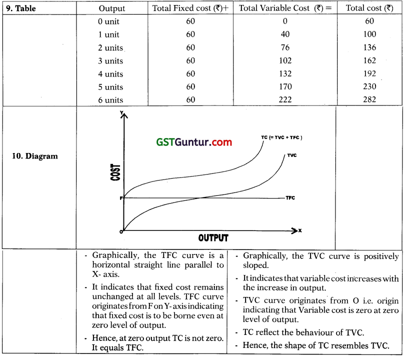
Short Run Total Costs:
Total Cost (in short run) = Total Fixed Cost + Total Variable Cost

Points	Fixed Cost	Variable Cost
1. Meaning	1. Fixed costs are incurred on the use of the fixed inputs. 2. Fixed inputs cannot be varied in the short run. 3. Therefore, fixed costs do not change with changes in output in short run. 4. Fixed costs are thus, Independent of output. 5. These include both Explicit Costs and Implicit Costs.	1. Variable costs are incurred on the use of the variable inputs. 2. Variable inputs can be varied in the short run. 3. Therefore, variable costs changes with the changes in output i.e. they increase or decrease when output rises or falls. 4. Variable costs thus, DEPEND on output.
2. Can Be Zero Or Not?	1. Fixed cost can never be zero. 2. If the level of output falls to ZERO, fixed costs are to be incurred in the short run. 3. In other words, if firm closes down for some time in short run but remains in business, these costs have to be borne by it	1. Variable cost can become zero. 2. If the level of output falls to zero, variable costs also falls to zero. 3. In other words, if a firm shuts down for some time in short run, it will not incur any variable cost as it will not use variable factors of production.
3. Examples	Example – Contractual rent, maintenance cost, property taxes, interest on capital invested, wages of permanent staff, depreciation, etc.	Example – wages of labour employed, prices of raw materials, power and fuel, expenses on transport, etc.
4. Determinant Factors	The examples of fixed cost above have no bearing on the volume of production.	1. The examples of variable cost above are closely related to the volume of production. 2. Hence variable costs are the determinant factor.
5. Relation With Output	Fixed cost have no relation with output in short run because these costs remain constant whatever be the level of output.	1. Variable costs are positively related with output. 2. If output is zero, variable cost is also zero. 3. If output is increased variable cost also rises FIRST at diminishing rate due to increasing return to factor AND THEN at an increasing rate due to diminishing returns to factor.
6. Function Of ?	Fixed Costs are therefore function of TIME.	Variable Costs are therefore function of Output.
7. Price Determination	In short run, the firm do not bother about recovering the fixed costs as it has to bear these costs even at zero level of output.	1. In short run, the firm must recover the variable costs to remain in business. 2. In other words firm’s Average Revenue ≥ Average Variable cost
8. Other Names	1. Fixed costs are also known as Over Head Costs as these costs are common to all the units of commodity produced. 2. They are also known as Supple Mentary Costs because the volume of output produced does not directly depend upon them.	Variable costs are also known as Prime or Direct Costs as all the units produced depend directly on them.

Semi Variable Cost:
Stair-step Variable Cost – Short run average cost:
→ For the purpose of making decisions about operations, unit cost functions or average costs are more useful than the total cost functions.

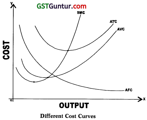
→ We examine here three of these unit cost functions namely –

• Average Fixed Cost (AFC),
• Average Variable Cost (AVC),
• Average Total Cost (ATC).

1. Average Fixed Cost:
→ Average Fixed Cost is the fixed cost per unit of output. Thus,
→ Average Fixed Cost = \(\frac { Total Fixed Cost }{ Total Output }\)
→ OR AFC = \(\frac { TFC }{ Q }\)

→ The above table shows that as the output increases, AFC goes on falling.

→ The reason being TFC is spread over larger quantities of output.

→ When graphed, the AFC curve slopes downwards from left to right throughout its length.

→ The AFC curve comes closer and closer to the X – axis but not touch the X-axis as TFC can never be zero.

→ AFC curve will not touch Y-axis also because at zero level of output, TFC is a Positive value. Any positive value divided by zero will provide infinite value.

→ The AFC curve is a Rectangular hyperbola because mathematically it shows the same level of TFC at all its points and geometrically the area of every rectangle on this curve at all points will be equal to the area of every other rectangle.

2. Average Variable Cost:
→ Average variable Cost is the variable cost per unit of output. Thus,
→ Average variable Cost = \(\frac { Total Variable Cost }{ Total Output }\)
→ OR AVC = \(\frac { TVC }{ Q }\)

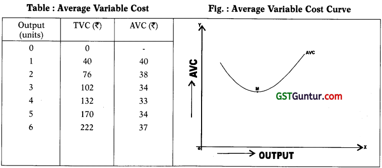
→ The above table shows that as the output expands, average variable cost falls initially due to increasing returns to the variable factor.

→ It is minimum at the optimum capacity output.

→ Beyond optimum capacity average variable cost rises very sharply due to diminishing returns to variable factor.

→ Thus, AVC and Average product of variable factor are inversely related.

→ When graphed, AVC curve declines over some range of output, reaches the minimum at optimum capacity, as at point ‘M’ in the above diagram and then goes on rising as output increases.

→ Thus, AVC curve is U-shaped indicating three phases decreasing phase, constant phase and increasing phase corresponding to the three phases of Average product of variable factor in the law of Variable Proportions.

3. Average Total Cost: {Or Simply Average Cost): .
→ Average Total Cost is the cost per unit of output. Thus,
→ Average Total Cost or Average Cost = \(\frac { Total Cost }{ Total Output }\)
→ ATC or AC = \(\frac { TC }{ Q }\)
→ ATC or AC = \(\frac { TFC }{ Q }\) + \(\frac { TVC }{ Q }\)
→ A TC or AC = AFC + AVC

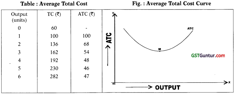
→ The above table shows that as output increases, ATC falls initially, reach its minimum and then rises due to the Law of variable proportions.

→ Since, ATC = AFC + AVC, it follows that the behaviour and shape of the ATC curve depends upon the behaviour of AVC curve and AFC curve.

→ In the beginning, the ATC curve falls sharply when output expands. REASON being, initially both AVC and AFC curves fall.

→ When AVC curve starts rising, but AFC curve continue to fall steeply, the ATC will continue to fall. REASON being, fall in AFC curve is MORE than the RISE in AVC curve.

→ As output further increases, ATC curve rises. REASON being, there is sharp rise in AVC which offsets the, fall in AFC. Thus, ATC curve first fall, reach its minimum and then rise.

→ Therefore, ATC curve is ‘U’- shaped for the same reasons for which the AVC is a ‘U’ – shaped curve.

4. Marginal Cost.
→ Marginal Cost is addition to the total cost caused by producing one more unit of output.

→ Thus, marginal cost is the cost of the additional unit of output.

→ It is measured by the change in total cost resulting from a unit increase in output. Thus,
MC_n = TC_n – TC_n-1 Or MC = \(\frac { ∆ TC }{ ∆Q }\) where, ∆ = change

→ Example – If 5 units are produced, total cost = ₹ 206
If 6 units are produced, total cost = ₹ 236
Marginal Cost of 6th unit of output = ₹ 30

→ The Marginal Cost is Independent of Fixed Cost.

→ In the short period, total fixed cost are constant for all levels of output.

→ The only change in total cost when output changes is Change in Variable Cost. Hence, marginal cost is affected only by the variable cost.

→ Therefore, marginal cost can also be defined as a change in TVC as a result of a unit change in output. This can be proved as follows –
MC_n = TC_n – TC_n-1
since, TC = TFC + TVC
MC_n = (TVC_n + TFC _n) – (TVC _n-1 + TFC _n-1 )
= TVC_n + TFC_n – TVC _n-1 – TFC _n-1.
= TVC_n – TVC_n-1

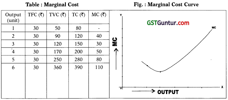
→ The above table shows that as the output increases, MC initially falls due to increasing returns to factor but finally MC rises due to diminishihg returns to factor.

→ Thus, marginal cost is the inverse of the marginal product of the variable factor.

→ When graphed, the MC curve first declines, reaches minimum and then goes on rising as output increases.

→ Thus, MC curve is U – shaped, this is due to the operation of the law of returns to factor and due to TC or TVC (AC or AVC).

→ MC curve passes through the minimum points of AVC and ATC curves

→ MC curve reaches its minimum point earlier to the minimum points of AVC and ATC curves.

Relationship between Average Cost and Marginal Cost:
→ Average Total Cost or Average Cost is the Cost per unit of output. Thus,
Average Total Cost = \(\frac { Total Cost }{ Total Output }\)
or AC = \(\frac { TC }{ Q }\)

Example – Suppose the total cost of producing 5 units of a commodity is ₹ 230, then average cost will be \(\frac { ₹ 230 }{ 5 units }\) = ₹ 46

→ Marginal Cost is addition to the total cost caused by producing one more unit of output. Thus, marginal cost is the cost of the additional unit of output. Symbolically, .
MC_n = TC_n – TC_n-1
Example – The total cost of producing 5 units is ₹ 206 and that of 6 units is ₹ 236. Then, marginal Cost of producing one more unit = ₹ 236 – ₹ 206 = ₹ 30.

→ The relationship between Average Total Cost and Marginal Cost can be illustrated with the help of following table and graph.
Table : Relationship between Average Cost and Marginal Cost

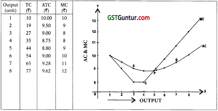
→ Both the table and diagram above bring out the relationship between average cost and mar-ginal cost clearly as follows:
1. Both AC and MC are derived from total cost of production. They are derived from the same source

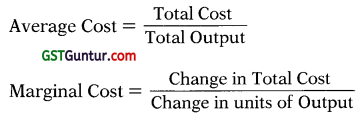
2.

• When average cost falls with increase in output, marginal cost also falls and is less than average cost.
• It means that marginal cost falls faster.
• Thus, when AC curve is falling, MC curve will be below AC curve.
• MC curve reaches minimum point ‘C’ earlier then AC curve.
• Then, MC curve start rising from point ‘C’ to point ‘P’ even when the AC curve is falling

3.

• The MC curve cuts the AC curve at its minimum point. ‘P’ in the diagram.
• It is the minimum point on AC curve i.e. point of optimum capacity where the average cost is minimum.
• Points ‘A’ and ‘B’ on the AC curve shows higher average cost due to under and over utilization of plant capacity at respective points..
• At point ‘P’ where the MC curve cuts the AC curve i.e. at point of optimum capacity, MC = AC.

4.

• When AC rises, with increase in output, MC also rises and is higher than AC. It means that MC rises faster.
• Thus, when AC curve is rising, MC curve will be above the AC curve.

5. At zero level of output, MC is indeterminate.

6. Between AC and MC, it is MC which brings about changes (i.e. rise or fall) in AC and not other way round.
Thus –

• When MC < AC, it pulls down AC and AC falls
• When MC = AC, AC is constant and at its minimum
• When MC > AC, it pulls up AC and AC rises.

7. The concept of MC is more significant in finding out equilibrium output while that of AC in finding profit and loss.

Long Run Average Cost Curve :

• Long run is a period of time during which the firm can vary all inputs.
• In short run we have seen that, some inputs are fixed and others can be varied to increase the level of output.
• But in long run all inputs are variable.
• In the short run, the size of the plant is fixed. The size of plant cannot be increased or reduced.
• However, in the long run the firm has sufficient time to bring about changes in the size of plant (i.e. machinery building etc.) in order to expand or contract output.
• Thus, in the long run the firm moves from one plant to another. It can increase the size of plant to increase its output or can have smaller plant if it has to reduce output.
• The long run average cost curve shows the minimum possible average cost for producing various levels of output.
• Consider the following figure –
  
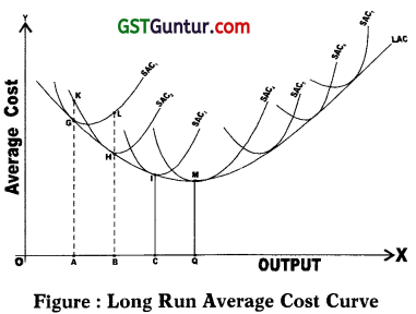
• In the fig., a smooth long run average cost curve has been shown which has been labelled as LAC.
• The LAC curve envelopes infinite short run average cost curves each representing a plant. Hence, SACs are also called plant curves.
• In the fig., the LAC curve is derived as a tangent to all the short run average cost curve from SAC₁ to SAC₇.
• Thus, it is U- shaped.
• In the long run, a firm can produce a particular output by building a relevant size of plant and operate on the corresponding SAC.
• It selects that size of plant i.e. SAC which gives the lowest cost of producing the given output.
• In the fig., seven short run average cost curves SAC₁, to SAC₇ corresponding to seven different plants are drawn.
• In the fig., if the firm wants to produce OA level of output, it will operate on SAC₁ at a cost of AG per unit.
• If the firm produce OA level of output with SAC₂ it will cost AK per unit to produce which is more.
• Similarly, if the firm wants to produce OB level of output with SAC₁ it will cost more i.e. BL per unit.
• So the firm to produce OB output will have to increase the size of plant and operate with SAC₂ where the cost per unit is less i.e. BH per unit.
• Thus, larger outputs can be economically produced i.e. at lowest cost with the bigger plants and small output can be economically produced i.e. at lowest cost with smaller plants.
• In the fig., OQ is the optimum output as it is being produced at the minimum point of LAC and corresponding SAC i.e. SAC₄. Thus, the long run average cost is minimum at output OQ.
• If the firm is producing less than optimum output OQ, the other plants are underutilized than their full capacity.
• If the firm is producing more than optimum output OQ, the other plants are overutilized than their full capacity.
• The fig., shows that LAC curve is not tangent to the minimum points of the SAC curves.
  → When LAC curve is sloping downwards, it is tangent to falling portions of SACs.
  → When LAC curve is rising upwards, it is tangent to rising portions of SACs.
• LAC curve is also called planning curve. Thus is because firm plans output in the long run but operates in the short run i.e. by choosing a plant on LAC corresponding to the given output.
• Thus, LAC helps the firm to make choice about the size of plant for producing a particular output at minimum cost.
• However, modern firms face ‘L’ shaped cost curve.

Why Long Run Average Cost Curve is of U-shape?

• As seen in the fig., LAC curve is U-shaped.
• The shape of LAC curve depends on the Law of Returns to Scale.
• As the firm expands, there is increasing returns to scale which means fall in long run average cost due to economies of scale.
• When decreasing returns to scale occur it means rise in long run average cost due to diseconomies of scale.
• This explains why LAC curve is U-shaped.