Time Series – CA Foundation Statistics Solutions

Time Series – CA Foundation Statistics Notes is designed strictly as per the latest syllabus and exam pattern.

Time Series – CA Foundation Statistics Notes

MEANING:- Most of the economic, Business and commerce data are recorded overtime i.e. the data relating to production; population; sales of products; bank deposits; profits; quantity of money in circulation etc., such data is called “time series data”.

Definition:- A series of statistical observations recorded overtime; usually at equal time interval is called “Time Series”.

According to Morris Hamburg: Aset of statistical observations arranged in chronological order i.e. usually equally time interval, is called Time Series.

According to Ya-Lun-Chou : A time series may be defined as a collection of magnitudes belonging to different time periods, of some variable or composite of variables such as production of steel; per capita income; gross national product; price of tobacco, or index of industrial production.

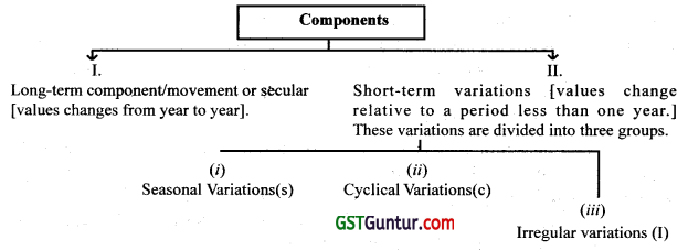
Components of Time Series

In the series of observations; we observe that the observations; we observe that the observations change form year to year; month to month and day to day. These changes are on account of a group of causes are called “components” or “factors” of time series.

Combining “Long Term” and “short-term variations together components/categories of Time Series are:-

(i) Long term components/movement or Secular trend/Simple trend (T)
(ii) Seasonal variations (S)
(iii) Cyclical variations (C)
(iv) Random or Irregular variations (I)

I. Secular/simple trend/long term movement

“The general tendency of a data is to increase or decrease or stagnate over a long period of time is called Secular trend or Simple trend.

Ex-Population of a country has increasing trend over years. Agricultural and Industrial production is increasing but health facilities, death rate is decreasing due to the use of modem technologies. Such types of many forces gradually act on time series variables to move in any direction over long period of the time.

II. Seasonal Variation

Those variations which complete within a year is called seasonal variations.

These variables are found in many historical series for which quarterly; monthly; weekly…. values are obtained. The main reason for seasonal variations are different climatic conditions in the year like festivals; customs and holidays. Industries related to agricultural products, soft drinks; ice cream; woolen garments; fashion; tourism; construction activities etc. are also affected by seasonal variations. Festivals like Diwali, Eid etc. also cause the sale of number of items to rise. Similarly in summer break for schools and colleges; great rush begins for Tour and Travels, Hotel, Resorts, Transports.

Seasonal variation is the most important component is used for future forecasting and planning in Time Series.

III. Cyclical Variations :-

In Economic and Commercial data, it has been observed that in addition to secular trend a regular upward and downward tendency is seen at the intervals between 7 to 11 years. This period sometimes may be peculiar to a particular industry but generally they more relate to the whole Economy and are called business cycles.

There are four phases of a business cycle. A peak time, known as prosperity or the boom, is followed by a decline (Recession) which intends to a low print or tough, which is sometimes called depression, depending on its degree of seriousness. The Trough is followed by a phase of recovery which is also known as expansion. This leads to a new peak and the cycle again begins.

IV. Irregular or Random Variations:-

Those variations observed in a set of time series which are not in the nature of trend or seasonal or cyclical variations are called Irregular or Random Variations. Due to unpredictable forces like a flood; tsunami, earthquake, labour strike etc. the irregular variations occur. These cause very deep downward or very high upward peak of the trend. It does not repeat in a definite pattern, so it cannot be predicted in advance.

Models of Time Series

Time series has two models which are generally used to decompose into its four components, Secular trend (T); Seasonal variation (S); Cyclical variation (C) and Irregular variation (I). The main objective of the time series is to estimate the relative impact of each component on the overall behaviour of the time series.

Models are

(i) Additive model
(ii) Multiplicative model

I. Additive model In this model; it is assumed that all four components are independent of each other. It means the pattern of occurrence and magnitude of the time series (Y) is defined as Y_t = T + S + C + I.

II. Multiplicative modelIn this model all four forces are assumed interdependent. It means, one the forces which are responsible for one type of variations are also responsible for other type of variations. That why the multiplication model occurs. This model is more suitable in business and Economic Time Series data. In this
case magnitude of time series is Y_t = T × S × C × I.

Example.
Let the Secular trend is ₹ 2,000, the Seasonal factor is ₹ 150 (i.e. it is expected to be ₹ 150 over the trend), the Cyclical factor is ₹ 80 (expected to depress ₹ 80) and Irregular factor ₹ 41 (Due to unpredictable random variation). Using additive model find monthly sales.
Solution:
Given that: T = ₹ 2,000; S = ₹150 ; C = ₹ 80 and I = ₹ 41.
∴ Monthly sales trend = Y_t = T + S + C + I.
= 2000 + 150 – 80 + 41 = ₹ 2,111

Example.
Let secular trend value of a commodity is ₹ 5,000; Due to seasonal variation sales up by 15% and cyclical factor is 0.90 (i.e. 10% reduction is sales) Residual factor is 1.03 (i.e. random rise by 3%). Estimate monthly sales.
Solution:
Here multiplicative model is suitable.
Estimated monthly sales = 5000 × 1.15 × (0.90).(1.03)
= ₹ 5330.25
Measurement of secular trend

Methods to find secular trend are :

(i) Graphic or a freehand curve method.
(ii) Method of semi Averages.
(iii) Method of moving averages
(iv) Method of least square.

(i) Graphic or freehand curve method

The Graphic presented of time series is also known as Line diagram or Histogram/ Histogram. It is the simplest method to study trend line. In this presentation; time is taken on X-axis and value of the variable on Y-axis.
Illustration Fit a trend line to the following data by freehand method :

Years	2005	2006	2007	2008	2009	2010	2011
Profit “in lakhs”	11	16	13	17	14	18	15

Solution.

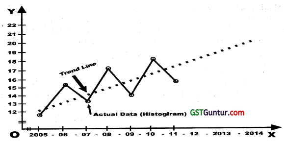
If trend values are obtained mathematically then these values are approximately close to the trend fitted by freehand method.

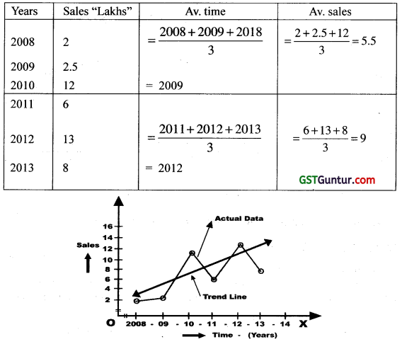
(ii) Method of Semi-Averages

In this method, the data is divided into two parts, preferably with the same no. of years

Case I: If the number of years is even; then average of time and value of the 1st half is determined and average of time and value of the rest half part is also determined.

We find the co-ordinates of time and value of both part on the graph and we join those points with scale and that straight line gives us the required trend line by semi-average method.

Illustration :-
Fit a trend line by semi-average method of the following data.

Years	2008	2009	2010	2011	2012	2013
Sale (“in lakhs”)	2	25	12	6	13	8

Solution:

Case II: If No. of years is odd.

In this case middle year and its value are ignored. Average of times and values of the upper part is determined and average of times and values of the lower part is also obtained. We get the trend line on the graph after joining these two points.

Illustration:-
Find trend values of the following data by method of semi-aver-ages

Years	2010	2011	2012	2013	2014	2015	2016
Profit (lakhs)	55	80	65	90	75	115	55

Solution:

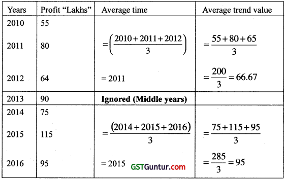
Co-ordinate of trend values are (2011; 66.67) and (2015 ; 95)

Method of moving averages

The method of moving averages is an important tool and is used to get trend values. It consists in averaging out seasonal variations and other short-terms variations from the time series. In this method, we have to consider following some points

1. Number of years (Even i.e. 2, 4, 6, etc. or odd 3, 5, 7 etc.) are taken into account.
2. Which type of averages (simple mean or weighted mean) are consider.

To find moving average trend values, following steps are taken under account.

(a) No. of years for moving averages may be even i.e. 2, 4, 6 etc. or 3, 5, 7 etc. It depends upon the cycle length.

(b) In case of “3-yearly moving average”; first we find average time of 1st 3yrs and their average value by dividing total by 3. It is written against the average time i.e. middle time. Then, we leave 1st year and go ahead
one more year. Leaving 1st year, again we find average time and average trend value like above and put the obtained trend value against the middle year. This process is continued until the value of last year is taken into account. In the case of even no. of years, average value obtained after dividing the total values by no. of years and put it against the mid value of the middle two years. Remaining process remains the same as in the case of odd no. of years.

(c) In case of even numbers of years average value does not correspond to a particular years. So, averages are re-averaged by taking two averages and put it against the corresponding year, this average is called centered value.

Illustration:-
Find 3-yearly moving average trend values of the following data. Years 2012 2013 2014 2015

Years	2012	2013	2014	2015	2016	2017	2018
Value	3	9	7	12	15	11	20

Solution:

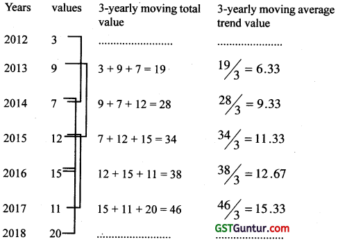
Illustration:-
Find 3-yearly weighted moving average Trend value of the following data taking weights of the 3

Years	2014	2015	2016	2017	2018
Value	7	12	10	15	20

Solution:
We know; weighted mean \(\overline{X_w}\)
\(\overline{\mathrm{X}_w}\) = \(\frac{\sum \mathrm{WX}}{\sum \mathrm{W}^{\prime}}\); Where x = value ; w = weight of values.

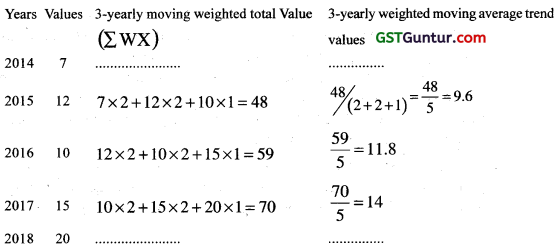
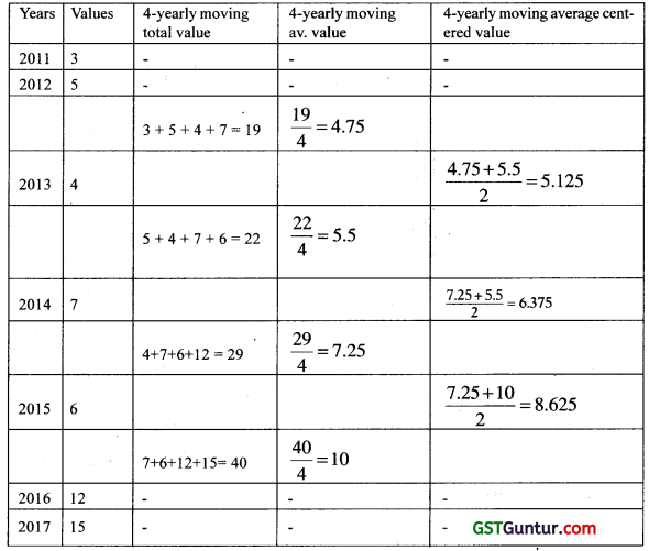
Illustration:-
Find 4-yearly moving average trend values of the following data.

Years	2011	2012	2013	2014	2015	2016	2017
Values	3	5	4	7	6	12	15

Solution:

Method of least square method

When we draw trend line graph by freehand method; we get two types of lines

(i) Straight Trend line or Linear Trend line &

(ii) Non-Linear Trend line (Qua-dratic trend line) Straight trend line Eqn. in Time Series is obtained by Least Square Method just like we studied in Regression Analysis. We know, Regression Trend line eqn. is assumed as Y = a + bx
Where a & b are constants.

In time series, Eqn. of the Linear Trend line is taken as Y = a + bx
Where a = Y – intercept
b = Slope of the trend-line.
X = Deviation of the time/year from base time/year.
X = [Current year – Base year.]

Note:- In Question; if base year is not mentioned then middle year of the data is taken as the base year.
Let Linear Trend Line eqn. is Y = a + bx

To find the values of two constant a & b; two normal Eqns. are taken.
They are –
ΣY = aN + bΣx
ΣXY = aΣX + bΣX²
Where N = No. of years
When middle year is taken as base year, then
ΣX = 0 [Always]
& a = \(\frac{\sum Y}{N}\) and b = \(\frac{\sum X Y}{\sum X^2}\)

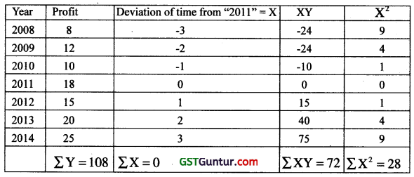
Illustration:-
Fit a straight trend line to the following data and estimate the profit for the year 2018.

Years	2008	2009	2010	2011	2012	2013	2014
Profit “000”	8	12	10	18	15	20	25

Solution:
Here we should take middle year 2011 as the base year because base year is not given.

Let the eqn. of the straight trend line is Y = a + bx
Its normal eqns. are
ΣY = aN + bΣx —– (i)
ΣXY = aΣx + bΣx² ——- (ii)
From(1); 108 = a × 7 + b × 0 ⇒ a = \(\frac{108}{7}\) ⇒ a = 15.43
From (2);
ΣXY = aΣX + bΣX²
72 = a × 0 + b × 28
or b = \(\frac{72}{28}\) = 2.57
Hence, the required Linear Trend line Eqn. is Y = 15.43 +2.57.X.
For year 2018; X = 2018 – 2011 = 7
Hence, estimated trend value for year 2018 is Y = 15.43 + (2.57).(7) = ₹ 33.42 thousand.
= ₹ 33,420.

Illustration:-
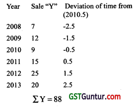
Fit a straight line trend to the following data by least square method. Find estimated sale for the year 2017.

Year	2008	2009	2010	2011	2012	2013
Sale (Lakhs)	7	12	9	15	25	20

Solution:
Here N = No. of years = 6 ( Even)
Let Base year = \(\frac{2010+2011}{2}\) = 2010.5
Let Linear Trend line Eqn. is Y = a + bx
Its Normal Eqns. are
ΣY = aN + bΣx ;
ΣXY = aΣx + bΣx²

From 1st Normal Eqn.
ΣY = aN + bΣx
88 = a × 6 + b × 0 ⇒ a = \(\frac{88}{6}\) = 14.67
From 2nd Normal Eqn.
aΣx + bΣx² = ΣXY
or a × 0 + b × 70 = 110
or b = \(\frac{110}{70}\) = 1.57
Hence, the required linear trend line eqn. is
Y= 14.67+ 1.57 X.
For year 2017
X = 2.(2017 – 2010.5) = 13
Estimated sale for the year 2017 is
Y_c = 14.67 + 1.57 × 13 = Rs.35.08 Lakhs
= ₹ 35,08,000.

Previous Year Exam Questions

Question 1.
The multiplicative time series model is [1 Mark, May 2018]
(a) Y = T + S + C + I
(b) Y = TSCI
(c) Y = a + bx
(d) Y = a + bx + cx²
Solution :
(b) Y = TSCI
The multiplicative time series model is
Y = TSCI
Where T ⇒ Trend Variation
S ⇒ Seasonal Variation
C ⇒ Cyclical Variation
T ⇒ Irregular Variation

Question 2.
The Simple Average Method is used to calculate [1 Mark, Nov. 2018]
(a) Trend Variation
(b) Cyclical Variation
(c) Seasonal Variation
(d) Irregular Variation
Solution:
(c) Seasonal Variation

Question 3.
The sale of Cold Drink would go up in summers and go down in the winters is an example of [1 Mark, Nov. 2018]
(a) Trend Variation
(b) Cyclical Variation
(c) Seasonal Variation
(d) 200
Solution:
(c) Seasonal Variation

Question 4.
In semi averages method, if the number of values is odd then we drop : [1 Mark, June 2019]
(a) First value
(b) Last value
(c) Middle value
(d) Middle two value
Solution:
(c) Middle value

Question 5.
Trend in semi averages is [1 Mark, June 2019]
(a) Linear
(b) Parabola
(c) Exponential
(d) None
Solution:
(a) Linear

Question 6.
The most commonly used Mathematical Method for finding Secular Trend is [1 Mark, June 2019]
(a) Moving average
(b) Simple average
(c) Exponential
(d) None
Solution:
(b) Simple average