Standard Costing – CA Final SCMPE Study Material

Standard Costing – CA Final SCMPE Study Material is designed strictly as per the latest syllabus and exam pattern.

Standard Costing – CA Final SCMPE Study Material

Question 1.
(Traditional, Planning and Operational Variance)

Required:
Calculate Traditional Variances, Operational Variances, Planning Variance
Answer:
Traditional Variances:
Usage Variance = (9,000 Kgs. – 8,750 Kgs.) × ₹ 12.50
= ₹ 3,125 (F)
Price Variance = (₹ 12.50 – ₹ 13.00) × 8,750 Kgs.
= ₹ 4,375 (A)
Total Variance = ₹ 3,125(F) + ₹ 4,375 (A)
= ₹ 1,250 (A)

Operational Variances:
Usage Variance = (10,125 Kgs. – 8,750 Kgs.) × ₹ 11.50
= ₹ 15,812.50 (F)
Price Variance = (₹ 11.50 – ₹ 13) × 8,750 Kgs.
= ₹ 13,125 (A)
Total Variance = ₹ 15,812.50 (F) + ₹ 13,125 (A)
= ₹ 2,687.50 (F)

Planning Variances:
Usage Variance = (9,000 Kgs. – 10,125 Kgs.) × ₹ 12.50
= ₹ 14,062.50 (A)
Price Variance = (₹ 12.50 11.50) × 10,125 Kgs.
= ₹ 10,125 (F)
Total Variance = ₹ 14,062.50 (A) + ₹ 10,125 (F)
= ₹ 3,937.50 (A)

Question 2.
(Revising the budget)
Roshan Co. manufactures Stopers which it is estimated require 2 kg of material LMN at ₹ 10/kg. In week 21 Budget is to produce 250 Stoppers. 450 kg of LMN were purchased and used in the week at a total cost of ₹ 5,100. Later it was found that the standard had failed to allow for a 10% price increase throughout the material supplier’s industry. Roshan Co carries no stocks.
Required: Analyse the Planning and Operational Variance
Answer:
Planning and operational analysis
The first step in the analysis is to calculate:
(1) Actual Results
(2) Revised flexed budget (ex-post).
(3) Original flexed budget (ex-ante).

Question 3.
(Original and Revised Flexed Budgets)
Revising the budget A transport business makes a particular journey regularly, and has established that the standard fuel cost for each journey is 20 litres of fuel at ₹ 2 per litre. New legislation has forced a change in the vehicle used for the journey and an unexpected rise in fuel costs. It is decided retrospectively that the standard cost per journey should have been 18 litres at ₹ 2.50 per litre.
Required: Calculate the original and revised flexed budgets if the journey is made 120 times in the period.
Answer:
Original flexed budget:
120 × 20 × ₹2 = ₹ 4,800
Revised flexed budget:
120 × 18 × ₹ 2.50 = ₹ 5,400

Question 4.
(Planning and Operational Variance of Material Price and
Usage Variance)
(i) In the case of Material Purchase Price Variance, suppose the standard Price of Raw Material determined was ₹ 5.00 per unit, there is economic depression worldwide, so the price of raw material was estimated to change to ₹ 5.20.
the General Market Price per unit at the time of purchase was ₹ 5.18 on the purchase of sat 10.000 units of Ra w Material.
(ii) In the case of material Usage Variance, suppose the Standard Quantity per unit be 5 Kgs., Actual Production units be 250 and Actual Quantity of Material uses is 1,450kgs. Standard Cost of material per Kg. was ₹ 1. Because of shortage of Skilled Labour it was felt necessary to use Unskilled labour and that increased Material Usage by 20%. The variances to be computer to deal with the current environmental conditions will be:
Required:
Calculate Panning and operational Variance of Material Purchase Price Variance and Material Purchase Usage Variance.
Answer:
In this case the variances to be computed should be:
(i) Material Purchase Price Variance
Planning Variance:
= (Standard Price p.u – General market Price p.u.) × Actual Quantity Purchased
= (₹ 5.00 – ₹ 5.20) × 10,000 units = ₹ 2,000 (A)
Uncontrollable
Operational Variance:
= (General Market Price p.u. – Actual Price Paid p.u.) × Actual Quantity Purchased
= (₹ 5.20 – ₹ 5.18) × 10,000 units
= ₹ 200(F)

(ii) Material Usage Variance
Planning Variance*:
= (Original Std. Quantity in Kgs – Revised Std.) × Standard Price per Kg.
= (1,250 Kgs. – 1,500 Kgs) × ₹ 1
= ₹ 250 (A)
uncontrollable
Operational Variance (Controllable):
= (Revised Standard t Quantity in Kgs. – Actual Quantity Uses in Kgs.) × Std. Price per Kg.
= (1,500Kgs. – 1,450Kgs.) × ₹ 1 = Rs. 50(F)

Question 5.
(Planning and Operational Variance of Material Price and Usage Variance)
PWP company is manufacturing and selling a product ‘X’ in the market. Product ‘X’ requires product ‘D’ as an input raw material. The y Raw material ‘D’ had a standard direct material cost in the budget of 1 kg of material D @ ₹ 10 per kg which is ₹ 40 per unit of product ‘x’ manufactured.

Due to domestic riot supply of material to the market has disrupted, the average market price for Material D during the period was 11 per kg, and it was decided by the management of the company to revise the material standard cost to allow for this.
During this period company has manufactured 6,000 units of product X. They required 26,300 kg of Material D, which cost ₹ 2,78,780. For the purpose of further analysis company has appointed an expert.
Required ; Calculate:
(i) the material price planning variance
(ii) the material price operational variance and usage operational variance
Answer:
(i) The original standard cost was 4kg × ₹ 10 = ₹ 40,
The revised standard cost is 4kg × ₹ 11 = ₹ 44.
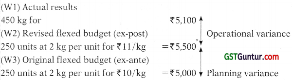
Material price planning variance
This is the difference between the original standard price for Material D and the revised standard price.

	₹ per kg
Original standard price	10.00
Revised standard price	11.00
Material price planning variance	1.00 (A)

The planning variance is adverse because the change in the standard price increases the material cost and this will result in lower profit.
The material price planning variance is converted into a total money amount by multiplying the planning variance per kg of material by the actual quantity of materials used.
Material price planning variance = 26,300 kg × ₹ 1.00 (A) = ₹ 26,300 (A).

(ii) Material price operational variance
This compares the actual price per kg of material with the revised standard price. It is calculated using the actual quantity of materials used.

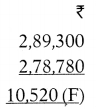
26,300 kg of Material should cost(revised standard ₹ 11) = 2,89,300
They did cost = 2,78,780
Material price operational variance = 10,520 (F)

Material usage operational variance:
This variance is calculated by comparing the actual material usage with the standard usage in the revised standard, and then it is converted into a money value by applying the original standard price for the materials.

	kg of D
6,000 units of Product × should use (4kg)	24,000
They did us	26.300
Material usage (operational) variance in kg of D	2,300 (A)
Original standard price per kg of Material D	₹ 10.00
Material usage (operational) variance in	₹ 23,000 (A)

The variances may be summarised as follows:

Question 6.
(Planning and Operational Variance)
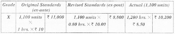
HDR Ltd produces units and incurs labour costs. A change in technology after the preparation of the budget resulted in a 25% increase in standard labour efficiency, such that it is now possible to produce 10 units instead of 8 units using 8 hours of labour-giving a revised standard labour requirement of 0.80 hours per unit. Details of actuals and budgeted for period XII are:

Required
(i) CALCULATE the variances for ‘X’ by
(a) Traditional Variance Analysis; and
(b) An approach which distinguishes between Planning and Operational Variances.
(ii) COMMENT on the results.
Answer:
(i) (a) Traditional Variances
Efficiency Variance = (1,100 hrs. – 1,200 hrs.) × ₹ 10
= ₹ 1,000 (A)
Rate Variance = (₹ 10 – ₹ 8.50) × 1,200 hrs.
= ₹ 1,800 (F)
Total Variance = ₹ 1,000 (A) + ₹ 1,800 (F) = ₹ 800 (F)

(b) Operational Variances
Efficiency Variance = (880 hrs. – 1,200 hrs.) × ₹ 10.00
= ₹ 3,200 (A)
Rate Variance = (₹ 10.00 – ₹ 8.50) × 1,200 hrs.
= ₹ 1,800 (F)
Total Variance = ₹ 3,200 (A) + ₹ 1,800 (F) = ₹ 1,400 (A)
Planning Variances
Efficiency Variance = (1,100 hrs. – 880 hrs.) × ₹ 10 = ₹ 2,200 (F)
Rate Variance = (₹ 10 – ₹ 10) × 800 hrs.
= ₹ 0
Total Variance = ₹ 2,200 (F) + ₹ 0 = ₹ 2,200 (F)

(ii) Comment
In this case, the separation of the labour cost variance into operational and planning components shows a large problem in the area of labour efficiency than might otherwise have been indicated. The operational variances are based on the revised (ex-post) standard and this gives a more meaningful performance benchmark than the original (ex-ante) standard.

Question 7.
(Planning and Operational Variance)
Managing Director of Petro-KL Ltd (PTKLL) thinks that Standard Costing has little to offer in the reporting of material variances due to frequently change in price of materials.
PTKLL can utilize one of two equally suitable raw materials and always plan to utilize the raw material which will lead to cheapest total production costs. However, PTKLL is frequently trapped by price changes and the material actually used often provides, after the event, to have been more expensive than the alternative which was originally rejected.
During last accounting period, to produce a unit of ‘P’ PTKLL could use either 2.50 Kg of ‘PG’ or 2.50 kg of ‘PD’. PTKLL planned to use ‘PG’ as it appeared it would be cheaper of the two and plans were based on a cost of ‘PG’of ₹ 1.50 per Kg. Due to market movements,
the actual prices changed and if PTKLL had purchased efficiently the cost would have been:
‘PG’ ₹2.25per Kg;
‘PD’ ₹2.00 per Kg
Production of ‘P’was 1,000 units and usage of ‘PG’amounted to 2,700 Kg at a total cost of t 6,480/-
Required
CALCULATE the material variance for ‘P’ by:
(i) Traditional Variance Analysis; and
(ii) An approach which distinguishes between Planning and Operational Variances. (10 Marks) [March 2019 MTP]
Answer:
(i) Traditional Variances (Actual Vs Original Budget)
Usage Variance = (2,500 Kg – 2,700 Kg) × ₹ 1.50
= ₹ 300(A)
Price Variance = (₹ 1.50 – ₹ 2.40) × 2,700 Kg
= ₹ 2,430 (A)
Total Variance = ₹ 300 (A) + ₹ 2,430 (A)
= ₹ 2,730 (A)

(ii) Operational Variances (Actual Vs Revised)
Usage Variance = (2,500 Kg – 2,700 Kg) × ₹ 2.25
= ₹ 450 (A)
Proce Variance = (₹ 2.25 – ₹ 2.40) × 2,700 Kg
= ₹ 405 (A)
Total Variance = ₹ 450 (A) + ₹ 405 (A)
= ₹ 855(A)

Planning Variances ‘
Controllable Variance = (₹2.00 – ₹2.25) × 2,500 Kg
= 625 (A)
Uncontrollable Variance = (₹ 1.50 – ₹2.00) × 2,500 Kg
= 1,250 (A)
Total Variance = ₹ 625 (A) + ₹ 1,250 (A)
= ₹ 1,875 (A)
Traditional Variance = Operational Variance + Planning Variance
Reconciliation
= ₹ 855 (A) + ₹ 1,875 (A)
= ₹ 2,730 (A)

Question 8:
(Planning and Operational Variance)
GRV is a chemical processing company that produces sprays used by farmers to protect their crops. One of these sprays ‘Agrofresh ’ is made by using either chemical A or chemical B. To produce one litre of Agrofresh spray they have the option to use either 12 litres of chemical A or 12 litres of chemical B. During the financial year, the purchase department of GRV has planned to use chemical B as it appeared that it would be the cheaper of the two and their plans were based on a cost of chemical B of ₹ 15 per litre.
Due to subsequent market movement during the year the actual prices changed and if the concerned department had purchased efficiently, the cost would have been

Chemical A	₹ 15.40 per litre
Chemical B	₹ 16.00 per litre

Production of Agrofresh spray was 1,000 litres and the usage of chemical B was 12,800 litres at a cost of ₹ 2,09,920.
You are the CEO of GRV and the Management Accountant has sent to you the following :
“I feel that in our particular circumstances the traditional approach to variance analysis is of little use as for some of our products we can utilize one of several equally suitable chemicals and we always plan to use such chemical which will lead to cheapest production costs. How’ever due to sharp market movements, we are frequently trapped by the sharp price changes which lead to the choice of expensive alternative at the end”
To check the reality in the content of the mail your CEO asked you, the cost accountant of the company:
(i) CALCULATE the material variance of Agi o Fresh by using
– Traditional Variance Analysis
– Planning and operational Variances (6 Marks)
(ii) ANALYSE how planning and operational variance approached the variances (2 Marks)
(iii) ANALYSE how the advanced variances at e useful to your organization (2 Marks) [May 2019 Exam]
Answer:
(i) Traditional Variances
Usage Variance = (12,000 It. – 12,800 It.) ₹ ₹ 15.00
= ₹ 12,000 (A)
Price Variance = (₹ 15.00 – ₹ 16.40) ₹ 12,800 It.
= ₹ 17,920 (A)
Total Variance = ₹ 12,000 (A) + ₹ 17,920 (A)
= ₹ 29,920 (A)

Operational Variances
Usage Variance = (12,000 1t. – 12,800 1t.) ₹₹ 16.00
= ₹ 12,800 (A)
Price Variance = (₹ 16.00 – ₹ 16.40) ₹ 12,800 It.
= ₹ 5,120 (A)
Total Variance = ₹ 12,800 (A) + ₹ 5,120 (A) = ₹ 17,920 (A)

Planning Variances
Controllable Variance = (₹ 15.40 – ₹ 16.00) ₹ 12,000 lt.
= ₹ 7,200 (A)
Uncontrollable Variance = (₹ 15.00 – ₹ 15.40) ₹ 12,000 lt.
= ₹ 4,800 (A)
Total Variance = ₹ 7,200 (A) + ₹ 4, 800 (A)
= ₹ 12,000 (A)
Reconciliation = ₹ 17,920 (A) + ₹ 12,000 (A) = ₹ 29,920 (A)
Direct Material Usage Operational Variance using Standard Price, and the Direct Material Price Planning Variance based on Actual Quantity can also be calculated. This approach reconciles the Direct Material Price Variance and Direct Material Usage Variance calculated in part.

(ii) Traditional variance analysis is applied based on the assumption that whole of the variance is due to operational deficiencies and the planning associated with setting the original standard is perfectly correct. But this assumption is not practical. When the conditions are volatile and dynamic, traditional variances need to be analysed into planning and operational variances. Planning variances try to explain the extent to which the original standard needs to be adjusted to reflect changes in operating conditions between the current situation and that imagined when the standard was originally derived. Planning variances are generally not controllable and may need to revise to cater the changes due to environmental/technological changes at a later stage. In certain situation planning variances can be considered controllable as well. Whereas operational variances explain the extent to which adjusted standards have been achieved. Operational variances are calculated after the planning variances have been established and are thus a realistic way of assessing performance. So, it Indicates a reality check of traditional variance analysis.

In GRV, as per traditional approach total variances are ₹ 29,920 (adverse), out of which ₹ 17,920 (adverse) accounts for total operational variance and ₹ 12,000 (adverse) is for total planning variance. It is necessary to analyse planning variances further. The planning variance of ₹ 12,000 (adverse) can be divided into an uncontrollable adverse variance of ₹ 4,800 and a controllable adverse variance of t 7,200. Similarly, total operational variance can be sub-classified as adverse price variance of ₹ 5,120 and adverse usage variance of ₹ 12,800. This analysis gives a clearer indication of the inefficiency of the purchasing function by the concerned department. Performance of the staff of the purchasing department should be evaluated/rewarded/based on variances which are controllable. If an adverse uncontrollable variance of ₹ 4,800 is reported in the performance reports this is likely to lead to dysfunctional motivation effects to the purchase department.

(iii) In today’s cutthroat competition managers must react quickly and accurately to the changes in technology, price fluctuation, consumer tastes, laws and regulations, economic conditions, political conditions, and international conditions etc. which are changing rapidly and dramatically. Accordingly, management accountant should be able to provide necessary inputs by a proper analysis of the things that pertains to his/her area like effect of changes in price. The unique features of advanced variance analysis are that, it considers different market conditions and changes in the dynamic environment.

Moreover, advanced variances classify variances into controllable and uncontrollable variances and helps the management to find out reasons for adverse variances so that corrective action can be taken. Similarly, if any adverse variances have arrived, because of changes in the market condition like inflation, it has to be differentiated from the other variances.

GRV is a type of organization where management of performance can be done only through advanced variance analysis. Advanced variance analysis of GRV shows that it has adverse planning variance as well as adverse operational variance. Further, the emergence of controllable and uncontrollable variances makes it a perfect case of advance variance analysis in GRV. In GRV, sharp price changes which lead to the choice of expensive alternative and efficiency of purchase department need to be analyzed, reported, and dealt separately by the joint effort of the management accountant and the top management. Hence, advanced variance analysis in GRV is an absolute necessity.

Question 9.
(Planning and Operational Variance)
Ski Slope had planned, when it originally designed its budget, to buy its artificial ice for ₹ 10/per kg. However, due to subsequent innovations in technology, producers slashed their prices to ₹ 9.70 per kg. and this figure is now considered to be a general market price for the purpose of performance assessment for the budget period. The actual price paid was ₹ 9.50, as the Ski Slope procurement department negotiated strongly for a better price. The other information relating to that period were as follows:

Required
(i) Calculate the variance for ice by
(a) Traditional Variance analysis; and
(b) An approach which distinguishes between planning and operational Variance
(ii) INTERPRET the result [May 2019 RTP]
Answer:
(i) (a) Traditional Variances
Usage Variance = (27,500 Kgs. – 27,225 Kgs.) × ₹ 10
= ₹ 2,750 (F)
Price Variance = (₹ 10 – ₹ 9.50) × 27,225 Kgs.
= ₹ 13,612.50 (F)
Total Variance = ₹ 2,750 (F) + ₹ 13,612.50 (F)
= ₹ 16,362.50 (F)

(b) Operational Variances
Usage Variance = (26,125 Kgs. – 27,225 Kgs.) × ₹ 9.70
= ₹ 10,670 (A)
Price Variance = (₹ 9.70 – ₹ 9.50) × 27,225 Kgs.
= ₹ 5,445 (F)
Total Variance = ₹ 10,670 (A) + ₹ 5,445 (F)
= ₹ 5,225 (A)

Planning Variances
Usage Variance = (27,500 Kgs. – 26,125 Kgs.) × ₹ 10
= 13,750 (F)
Price Variance = (₹ 10 – ₹ 9.70) × 26,125 Kgs.
= ₹ 7,837.50 (F)
Total Variance = ₹ 13,750 (F) + ₹ 7,837.5O (F)
= 21,587.50 (F)

(ii) Interpretation
It is important to note that an innovation in technology is outside the control of Ski Slope and is, by nature, a planning ‘error’. Equally, the better negotiation of a price should be recognized as an operational matter. Operational variances are self- evidently under the control of operational management, so operational efficiency must be assessed with only these figures in mind. The material procurement department has clearly done well by negotiating a price reduction beyond the market dip. One might question the quality of the ice, as the usage variance is adverse (possibly the ice fails to cover the field and so more is required). Obviously, the favourable price variance is mailer than the adverse usage variance, thus, overall performance is quite poor. A supervisor cannot assess variances in isolation from each other.

Question 10.
(Planning & Operational Variance)
KONY Ltd., based in Kuala Lumpur, is the Malaysian subsidiary of Japan’s NY corporation, headquartered in Tokyo. KONY’s principal Malaysian businesses include marketing, sales, and after-sales service of electronic products & software exports products. KONY set up a new factory in Penang to manufacture and sell integrated circuit ‘Q50X-N’. The first quarter’s budgeted production and sales were 2,000units. The budgeted sales price and standard costs for ‘Q50X-N’ were as follows:

	RM	RM
Standard Sales Price per unit		50
Standard Costs per unit
Circuit X (10 units @ RM 2.5)	25
Circuit Designers (6 hrs. @ RM 2)	12	(37)
Standard Contribution per unit		13

Actual results for the first quarter were as follows:

	RM’000	RM’000
Sales (2,000 units)		158
Production Costs (2,000 units)
Circuit X (21,600 units)	97.20
Circuit Designers (11,600 hours)	34.80	(132)
Actual Contribution (2,000 units)		26

The management accountant made the following observations on the actual results-
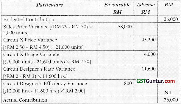
“In total, the performance agreed with budget; however, in eveiy aspect other than volume, there were huge differences. Sales were made at what was supposed to be the highest feasible price, but we now feel that we I could have sold for RM82.50 with no adverse effect on volume. The Circuit X cost that was anticipated at the time the budget was prepared was RM 2.5 per unit. However, the general market price relating to efficient purchases of the Circuit X during the quarter was RM 4.25 per unit. Circuit designers have the responsibility of designing electronic circuits that make up electrical systems. Circuit Designer’s costs rose dramatically with increased demand for the specialist skills required to produce the ‘Q50X-N’, and the general market rate was RM 3.125 per hour – although KONY always paid below the normal market rate whenever possible. In my opinion, it is not necessary to measure the first quarter’s performance through variance analysis. Further, our operations are fully efficient as the final contribution is equal to the original budget. ”
Required
COMMENT on management accountant’s view. [MAY 2020 RTP]
Answer:
Comment
As the management accountant states, and the analysis (W.N.1) presents, the overall variance for the KONI is nil. The cumulative adverse variances exactly offset the favourable variances i.e. sales price variance and circuit designer’s efficiency variance. However, this traditional analysis does not clearly show the efficiency with which the KONI operated during the quarter, as it is difficult to say whether some of the variances arose from the use of incorrect standards, or whether they were due to efficient or inefficient application of those standards.

As seen from W.N.3, on the cost side, the circuit designer’s rate variance has changed from adverse to favourable, and the price variance for component X, while remaining adverse, is significantly reduced in comparison to that calculated under the traditional analysis (W.N.l); on the sales side, sales price variance, which was particularly large and favourable in the traditional analysis (W.N.l), is changed into an adverse variance in the revised approach, reflecting the fact that the KONI failed to sell at prices that were actually available in the market.

Further, variances arose from changes in factors external to the business (W.N .4), which might not have been known or acknowledged by standard-setters at the time of planning are beyond the control of the operational managers. The distinction between variances is necessary to gain a realistic measure of operational efficiency.
W.N.l
KONY India Ltd.
Quarter-1

Operating Statement

W.N.2
Statement Showing Original Standards, Revised Standards, and Actual Results for Quarter 1

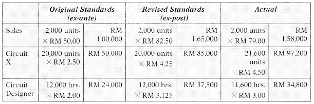
Original Standards (ex-ante) Revised Standards (ex-post) Actual
Sales 2,000 units X RM 50.00 RM
1,00,000 2,000 units X RM 82.50 RM
1,65,000 2,000 units X RM 79.00 RM
1,58,000
Circuit
X 20,000 unit s X RM 2.50 RM 50.000 20,000 units X RM 4.25 RM 85,000 21.600 units X RM 4.50 RM 97,200
Circuit
Designer 12,000 hrs. X RM 2.00 RM 24,000 12,000 hrs. X RM 3.125 RM .37,500 11,600 hrs. X RM 3.00 RM 34,800

W.N.3
Statement Showing Operational Variances

Particulars	(₹)	(₹)
Operational Variances		16,500 (A)
Sales Price [(RM 79.00 – RM 82.50) × 2,000 units]	7,000 (A)
Circuit × Price [(RM 4.25 – RM 4.50) × 21,600 units]	5,400 (A)
Circuit × Usage [(20,000 units – 21,600 units) × RM 4.25]	6,800 (A)
Circuit Designer Rate [(RM 3.125 – RM 3.00) × 11,600 hrs.]	1,450 (F)
Circuit Designer Efficiency [(12,000 hrs – 11,600 hrs.) × RM 3.125]	1,250 (F)

W.N.4
Statement Showing Planning Variances

Particulars	(₹)	(₹)
Planning Variance		16,500 (F)
Sales Price [(RM 82.50 – RM 50.00) × 2,000 units]	65,000 (F)
Circuit X Price [(RM 2.50 – RM 4.25) × 20,000 units]	35,000 (A)
Circuit Designer Rate [(RM 2.00 – RM 3.125) × 12,000 hrs.]	13,500 (A)

Question 11.
(Variance Analysis in Activity Based Costing)
N & S Co. (NSC) is a multiple product manufacturer. NSC pr oduces the unit and all overheads are associated with the delivery of units to its customers.

Particulars	Budget	Actual
Overheads (₹)	4,000	3,900
Output (units)	2,000	2,100
Customer Deliveries (no.’s)	20	19

Required
CALCULATE Efficiency Variance and Expenditure Variance by adopting ABC approach.
Answer:
Computation of Variances
Efficiency Variance = Cost Impact of undertaking activities more/less than standard
= (21 deliveries* – 19 deliveries) × ₹ 200
= ₹ 400 F
(*) $\left(\frac{20 \text { Deliveries }}{2,000 \text { units }}\right)$ ₹ 2,100 units.

Expenditure Variance = Cost impact of paying more/less than standard for actual activities undertaken
= 19 deliveries × ₹ 200 – ₹ 3,900
= ₹ 100 (A)

Question 12.
(Variance Analysis of ABC)
Raju is Chief Financial Officer of Millets, com, an internet company that enables customer to aider for delivery of different millets by accessing its website. Raju is concerned with the efficiency and effectiveness of the financial function. He collects the following information for three finance activities in 2021.
Rate per unit of Cost Driver

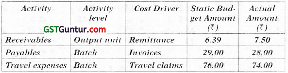
The output measure is the number of deliveries which is the same as the number of remittances. The following additional information are also given:

	Budgeted	Actual
Number of deliveries	10,00,000	9,48,000
Delivery Batch size	5	4.468
Travel expenses Batch size	500	501.587

Required
CALCULATE the flexible budget variances for 2021 to :
(i) Receivable Activities (2 Marks)
(ii) Payable Activities (4 Marks)
(iii) Travel expense Activities (4 Marks)
(Ignore fractions in all calculations) [May 2019 Exam]
Answer:
Activity-based costing, flexible-budget variances for finance function activities.
(i) Receivables
Receivables is an output unit level activity. Its flexible-budget variance can be calculated as follows:
Flexible Budget Variance = Flexible Budget Costs – Actual Costs
= ₹ 6.39 × 9,48,000 – ₹ 7.50 × 9,48,000
= ₹ 60,57,720 – ₹ 71,10,000
= ₹ 10,52,280 (A)

(ii) Payables
Payables is a batch level activity.

	Static-Budget Amounts	Actual Amounts
Number of deliveries	10,00,000	9,48,000
Batch size (units per batch)	5	4.468
Number of batches (a/b)	2,00,000	2,12,175
Cost per batch	₹ 29	₹ 28
Total payables activity cost (c × d)	₹ 58,00,000	₹ 59,40,900

Step 1: The number of batches in which payables should have been processed
= 9,48,000 actual units/5 budgeted units per batch
= 189,600 batches

Step 2: The flexible-budget amount for payables
= 1,89,600 batches × ₹ 29 budgeted cost per batch
= ₹ 54,98,400
The flexible-budget variance can be computed as follows:

Flexible-Budget Variance
= Flexible-Budget Costs – Actual Costs
= 1,89,600 × ₹ 29 – 2,12,175 × ₹ 28
= ₹ 54,98,400 – ₹ 59,40,900
= ₹ 4,42,500 (A)

(iii) Travel Expenses
Travel expenses is a batch level activity.

	Static-Budget Amounts	Actual Amounts
a. Number of deliveries	10,00,000	9,48,000
b. Batch size (units per batch)	500	501.587
c. Number of batches (a/b)	₹,000	1,890
d. Cost per batch	₹ 76	₹ 74
e. Total travel expenses activity cost (c × d)	₹ 1,52,000	₹ 1,39,860 ‘

Step 1: The number of batches in which the travel expense should have been processed
= 948,000 actual units/500 budgeted units per batch
= 1,896 batches

Step 2: The flexible-budget amount for travel expenses = 1,896 batches × ₹ 76 budgeted cost per batch
= ₹ 1,44,096

The flexible budget variance can be calculated as follows:
Flexible Budget Variance
= Flexible-Budget Costs – Actual Costs = 1,896 × ₹ 76 – 1,890 × ₹ 74 = ₹ 1,44,096 – ₹ 1,39,860
= ₹ 4,236 (F)

Question 13.
(Variance analysis of ABC)
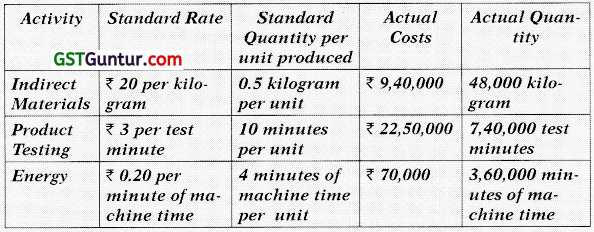
SPS Limited uses activity based costing to allocate variable manufacturing overhead costs to products. The company identified three activities with the following information for last quarter:

Required
(i) CALCULATE variable overhead expenditure variance and variable overhead efficiency variance for each of the activities using activity based costing. Clearly indicate each variance as favourable or unfavourable/adverse. (6 Marks)
(ii) INTERPRET the results of variable overhead efficiency variance as calculated in (i) above in respect of indirect materials and product testing activity. (2 Marks)
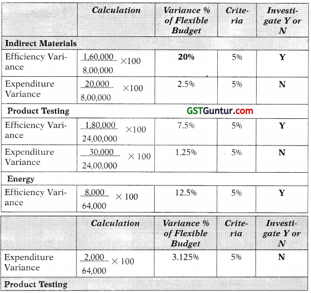
(iii) IDENTIFY the variances that should he investigated according to company policy. Show calculations to support your answer.
(2 Marks)
The company produced 80,000 units in the last quarter. Company policy is to investigate all variances above 5% of the flexible budget amount for each activity. [Nov. 2019]
Answer:
(i) Indirect Materials:
= Cost Impact of undertaking activities more/less than standard
= (0.50kg. × 80,000 units – 48,000 kg.) × ₹ 20
= ₹ 1,60,000 (A)

Expenditure Variance = Cost impact of paying more/less than standard for actual activities under- taken
= 48.000 kg. × ₹ 20 – ₹ 9,40,000
= ₹ 20,000 (F)

Product Testing
Efficiency Variance = Cost Impact of undertaking activities more/less than standard
= (10 mins. × 80,000 units – 7,40,000 mins.) × ₹ 3
= ₹ 1,80,000 (F)

Expenditure Variance = Cost impact of paying more/less than j standard for actual activities under-taken
= 7,40,000 mins × ₹ 3 – ₹ 2,50,000
= ₹ 30,000 (A)

Energy:
Efficiency Variance = Cost Impact of undertaking activities more/less than standard
= (4 mins. × 80,000 units – 3,60,000 mins.) × ₹ 0.20
= ₹ 8,000 (A)

Expenditure Variance = Cost impact of paying more/less than standard for actual activities undertaken
= 3,60,000 mins × ₹ 0.20 – ₹ 70,000
= ₹ 2,000 (F)

(ii) Indirect Materials
SPS actually spent 48,000 kg. or 8,000 kg. more than the standard allows. At a predetermined rate of ₹ 20 per kg., efficiency variance is 1,60,000 (A). Since actual quantity were higher than the standard, the variance is unfavourable. This adverse variance, could have been caused by the inferior quality, result of carelessness handling of materials by production workers or could as a result of change in methods of production, product specifications or the way in which quality of the product is checked or controlled.

Product Testing
Favourable efficiency variance amounting to ₹ 1,80,000 indicates that fewer testing minutes were expended during the quarter than the standard minutes required for the level of actual output. This may be due to employment of a higher skilled labour or improvement of skills of existing workforce through training and development leading to improved productivity etc.

(iii) Flexible Budget

Indirect Materials	= (0.50 kg. × 80,000 units) × ₹ 20 = ₹ 8,00,000	= ₹ 8,Q0,000 × 5% = ₹ 40,000
Product Testing	= (10 mins. × 80,000 units) × ₹ 3 = ₹ 24,00,000	= ₹ 24,00,000 × 5% = ₹ 1,20,000
Energy	= (4 mins. × 80,000) × ₹ 0.20 = ₹ 64,000	= ₹ 64,000 × 5% = ₹ 3,200

Efficiency Variance for all the three activities are more than 5% of their flexible budget amount. So, according to the company policy, efficiency variances should be investigated.

Alternative
Statement Showing Identification of Variances to be investigated

Question 14.
(Material, Labour Planning & Operational Variance, Variance Analysis of ABC)
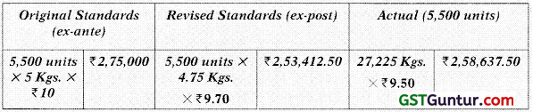
JPY Limited produces a single product. It has recently autotmated part of its manufacturing plant and adopted Total Quality Management (TQM) and Just-in- Time manufacturing system. No inventories are held for material as well as for finished product. The company currently uses standard absorption costing system. Following are related to fourth quarter of 2020-21;

	Budget	Actual
Production and Sales	1,00,000 units	1,10,000 units
Direct Materials	2,00,000 kg. @ ₹ 30/kg	2,50,000 kg. @ ₹ 31.20/kg.
Direct Labour Hours	25,000 hrs. @ ₹300/ hr	23,000 hrs. @ ₹ 300/ hr.
Fixed Production Overhead	₹ 3,20,000	₹ 3,60,000

Production overheads are absorbed on the basis of direct labour hours.
The CEO intends to introduce activity based costing system along with TQM and JIT for better cost management. A committee has been formed for this purpose. The committee has further, analysed and classified the production overhead of fourth quarter as follows:

	Budget	Actual
Costs:
Material Handling	₹ 96,000	₹ 1,24,000
Set Up	₹ 2,24,000	₹ 2,36,000
Activity:
Material Handling (orders executed)	8,000	8,500
Set Up (production runs)	2,000	2,100

Revision of standards relating to fourth quarter were made as below:

	Original Standard	Revised Standard
Material Content per unit	2 kg	2 .25 kg
Cost of Material	₹30 per kg	₹31 per kg
Direct Labour Hours	15 minutes	12 minutes

Required
(i) CALCULATE Planning and Operational Variances relating to material price, material usage, labour efficiency, and labour rate.
(ii) CALCULATE overhead expenditure and efficiency variance
using Activity Based Costing principles.
Answer:
(i) Workings

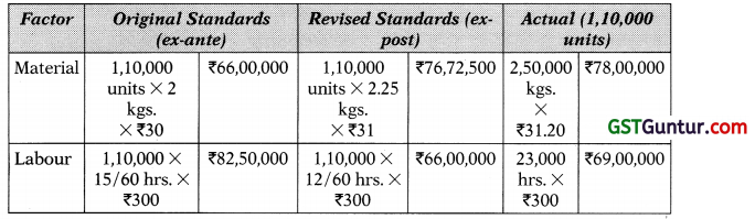
Material
Traditional Variances
Usage Variance = (2,20,000 Kgs. – 2,50,000 Kgs.) × ₹ 30
= ₹ 9,00,000 (A)
Price Variance = (₹ 30.00 – ₹ 31.20) × 2,50,000 Kgs.
= ₹ 3,00,000 (A)
Total Variance = ₹ 9,00,000 (A) + ₹ 3,00,000 (A)
= ₹ 12,00,000 (A)

Planning Variances
Usage Variance = (2,20,0000 Kg. – 2,47,500 Kg.) × ₹ 30
= ₹ 8,25,000 (A)
Price Variance = (₹ 30 – ₹ 31) × 2,47,500 Kgs.
= ₹ 2,47,500 (A)
Total Variance = ₹ 8,25,000 (A) + ₹ 2,47,5000 (A)
= ₹ 10,72,500 (A)

Operational Variances
Usage Variance = (2,47,500 Kg. – 2,50,000 Kg.) × ₹ 31
= ₹ 77,500 (A)
Price Variance = (₹ 31.00 – ₹ 31.20) × 2,50,000 Kg.
= ₹ 50,000 (A)
Total Variance = ₹ 77,500 (A) + ₹ 50,000 (A)
= ₹ 1,27,500 (A)
Direct Material Usage Operational Variance using Standard Price, and the Direct Material Price Planning Variance based on Actual Quantity can also be calculated. This approach reconciles the Direct Material Price Variance and Direct Material Usage Variance calculated in part.
Labour
Traditional Variances
Efficiency Variance = (27,500 hrs. – 23,000 hrs.) × ₹300
= ₹13,50,000 (F)
Rate Variance = (₹300 – ₹300) × 23,000 hrs.
= NIL
Total Variance = ₹ 3,50,000 (F) + NIL
= ₹ 13,50,000 (F)

Planning Variances
Efficiency Variance = (27,500 hrs. – 22,000 hrs.) × ₹ 300
= ₹ 16,50,000 (F)
Rate Variance = (₹ 300 – ₹ 300) × 22,000 hrs.
= NIL
Total Variance = ₹ 16,50,000 (F) + 0
= ₹16,50,000 (F)

Operational Variances =
Efficiency Variance = (22,000 hrs. – 23,000 hrs.) × ₹ 300
= ₹ 3,00,000 (A)
Rate Variance = (₹ 300 – ₹ 300) × 23,000 hrs.
= NIL
Total Variance = ₹ 3,00,000 (A) + 0
= ₹ 3,00,000 (A)
Direct Labour Efficiency Operational Variance using Standard Rate, and the Direct Labour Rate Planning Variance based on Actual Hours can also be calculated. This approach reconciles the Direct Labour Rate Variance and Direct Labour Efficiency Variance calculated in part.

(ii) Material Handling
Efficiency Variance = Cost Impact of undertaking activities more/less than Standard
= (8,800 orders* – 8,500 orders) × ₹ 12
= ₹ 3,600(F)
*(8,000 orders /1,00,000 units) × 1,10,000 units
Expenditure Variance = Cost impact of paying more/less than standard for actual activities undertaken
= 8,500 orders × ₹12 – ₹1,24,000
= ₹22,000 (A)

Setup
Efficiency Variance = Cost Impact of undertaking activities more/ less than standard
= (2,200 runs* – 2,100 runs) × ₹ 112
= ₹ 11,200 (F)
*(2,000 runs/1,00,000 units) × 1,10,000 units
Expenditure Variance = Cost impact of paying more/less than standard for actual activities undertaken
= 2,100 runs × ₹112 – ₹2,36,000
= ₹ 800 (A)

Question 15.
(Learning Curve Impact on Variance; Life Cycle Costing)
DK International is developing a new product. During its expected life, 16,000 units of the product will be sold for ₹ 102 per unit. Production will be in batches of 1,000 units throughout the life of the product.
The direct labour cost is expected to reduce due to the effects of learning for the first eight batches produced. Thereafter, the direct labour cost will remain constant at the same cost per batch as in the 8th batch.
The direct labour cost of the first batch of 1,000 units is expected to be ₹ 55,000 and a 90% learning effect is expected to occur. The direct material and other non-labour related variable costs will be ₹ 50 per unit throughout the life of the product.
There are no fixed costs that are specific to the product.
The learning index for a 90% learning Curve = – 0.152; 8^-0.152 = 0.729; 7^-0.152 = 0.744
Required
(i) CALCULATE the expected direct labour cost of the 8*h batch. (3 marks)
(ii) CALCULATE the expected contribution to be earned from the product over its lifetime. (3 marks)
(iii) CALCULATE the rate of learning required to achieve a lifetime product contribution of ₹ 5,00,000, assuming that a constant rate of learning applies throughout the product’s life. (4 marks) [May 2019 Exam]
Answer:
(i) Total Direct Labour Cost for first 8 batches based on learning curve | of 90% (when the direct labour cost for the first batch is ₹ 55,000)
The usual learning curve model is
y = ax^b
Where
y = Average Direct Labour Cost per batch for x batches
a = Direct Labour Cost for first batch
x = Cumulative No. of batches produced
b = Learning Coefficient/Index
y = ₹ 55,000 × (8)^-0.152
= ₹ 55,000 × 0.729
= ₹ 40,095
Total Direct Labour Cost for first 8 batches
= 8 batches × ₹ 40,095
= ₹ 3,20,760
Total Direct Labour Cost for first 7 batches based on learning curve of 90% (when the direct labour cost for the first batch is ₹ 55,000)
y = ₹ 55,000 × (7)^-0.152
= ₹ 55,000 × 0.744
= ₹ 40,920
Total Direct Labour Cost for first 7 batches
= 7 batches × ₹ 40,920
= ₹ 2,86,440
Direct Labour Cost for 8^th batch
= ₹ 3,20,760 – ₹ 2,86,440
= ₹ 34,320

(ii) Statement Showing “Life Time Expected Contribution”

Particulars	Amount (₹)
Sales (₹ 102 × 16,000 units)	16,32,000
Less: Direct Material and Other Non Labour Related Variable Costs (₹ 50 × 16,000 units)	8,00,000
Less: Direct Labour	5,95,320
Expected Contribution	2,36,680

(*) Total Labour Cost over the Product’s Life
= ₹ 3,20,760 + (8 batches × ₹ 34,320)
= ₹ 5,95,320

(iii) In order to achieve a Profit of ₹ 5,00,000 the Total Direct Labour Cost over the Product’s Lifetime would have to equal ₹ 3,32,000.
Statement Showing “Life Time Direct Labour Cost”

Particulars	Amount (₹)
Sales (₹ 102 × 16,000 units)	16,32,000
Less: Direct Material and Other Non Labour Related Variable Costs (₹ 50 × 16,000 units)	8,00,000
Less: Desired Life Time Contribution	5,00,000
Direct Labour	3,32,000

Average Direct Labour Cost per batch for 16 batches is ₹ 20,750 (₹ 3,32,000/16 batches).
Total Direct Labour Cost for 16 batches based on learning curve of r% (when the direct labour cost for the first batch is ₹ 55,000)
y = ₹ 55,000 × (16)^b
₹ 20,750 = ₹ 55,000 × (16)^b
0.3773 = (16)^b
log 0.3773 = b × log 2⁴
log 0.3773 = b × 4 log 2
log 0.3773 = $\frac{(\log r)}{(\log 2)}$ × 4 log 2
= log 0.3773 = log r⁴
0.3773 = r⁴
r = ⁴0.3773
r = 78.37%

Alternative:
In order to achieve a contribution of ₹ 5,00,000, the total labour cost over the product’s lifetime would have to be ₹ 8,32,000 – ₹ 5,00,000 = ₹ 3,32,000.This equals an average batch cost of ₹ 3,32,000/16 = ₹ 20,750/-. This represents ₹ 20,750/₹ 55,000 = 37.73% of the cost of the first batch.
16 batched represent 4 doublings of output.
Therefore, the rate of learning required = $\sqrt[4]{0.3773}$ = 78.37%

Question 16.
(Learning Curve Impact on Variance)
The learning curve as a management accounting has now become or going to become an accepted tool in industry, for its applications are almost unlimited. When it is used correctly, it can lead to increase business and higher profits; when used without proper knowledge, it can lead to lost business and bankruptcy. State precisely:
(i) Your understanding of the learning curve:
(ii) The theory of learning curve;
(iii) The areas where learning curves may assist in management accounting; and
(iv) Illustrate the use of learning curves for calculating the expected average units cost of making.
(a) 4 machines
(b) 8 machines
Using the data below:
Data:
Direct Labour need to make first machine = 1,000 hrs.
Learning curve = 90%
Direct Labour cost = ₹ 15 per hour.
Direct materials cost = ₹ 1,50,000
Fixed cost for either size orders = ₹ 60,000.
Answer:
Statement showing computation of cost of making 4 machines & 8 machines:

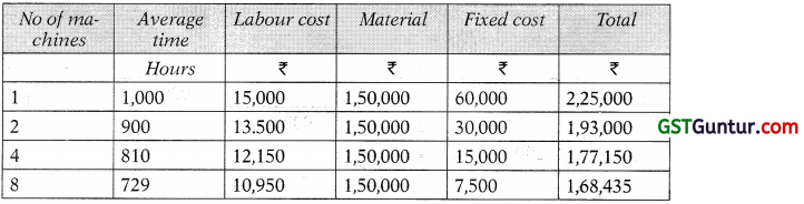
Average cost of making 4 machines ₹ 1,77,150
Average cost of making 8 machines ₹ 1,68,435

Question 17.
(Learning Curve Impact on Variance)
Z.P.L. C experience difficulty in its budgeting process because it finds it necessary to qualify the learning effect as new products are introduced. Substantial product changes occur and result in the need for retraining. An order for 30 units of a new product has been received by Z.P.L.C So far, 14 have been completed; the first unit required 40 direct labour hours and a total of 240 direct labour has been recorded for the 14 units. The production manager expects an 80% learning effect for this type of work.
The company use standard absorption costing. The direct costs attributed to the centre in which the unit is manufactured and its direct materials costs are as follows:

	₹
Direct material	30.00 per unit
Direct Labour	6.00 per hour
Variable overhead	0.50 per direct labour hour
Fixed overhead	6,000 per four-week operating period.

There are ten direct employees working a five-day week, eight hours per day. Personal and other downtime allowances account for 25% of total available time.
The company usually quotes a four-week delivery period for orders.
You are required to:
(i) Determine whether the assumption of an 80% learning effect 1 is a reasonable one in this case, by using the standard formula y = ax^b
Where Y = the cumulative average direct labour time per unit (productivity)
a = the average labour time per unit for the first batch,
x = the cumulative number of batches produced,
b = the index of learning.
(ii) Calculate the number of direct labour hours likely to be required for an expected second order of 20 units.
(iii) Use the cost data given to produce an estimated product cost for the initial order, examine the problems which may be created for budgeting by the presence of the learning effect.
Answer:
(i) Total time taken to produce 14 units
Y = ax⁶
Y = 40(14)^-0.322 = 17.14
Total time = 17.14 × 14 = 239.96 = 240 hours
It is true that learning ratio 80% is effective.

(ii) 30 units
Y = 40(30)^-0.322 = 13.3 80 hours (Average time)
50 units
Y = 40(50)^-0.322 = 1 1.35 hours (Average time)
Total time for 30 units = 13.38 × 30 = 401.4 hours
Total time for 50 units = 11.35 × 50 = 567.5 hours
Time taken for 20 units from 31 to 50 units (567.5 – 401.4) = 166.1 hours

(iii) Man hours = 10 × 8 × 5 × 4 = 1,600
(-) down time = 400.
= 1,200

Fixed Cost per hour = 6,000/1,200 = ₹ 5
Computation of total cost for the initial order
Material (30 × 30) = ₹ 900.0
Labour (401.4 × 6) = ₹ 2408.4
Variable Overheads (0.5 × 401.4) = ₹ 200.7
Fixed Overheads (5 × 401.4) = ₹ 2007.0
Total = ₹ 900.0 + ₹ 2408.4 + ₹ 200.7 + ₹ 2007.0 = ₹ 5516.1

Question 18.
(Learning Curve Impact on Variance)
A firm received an order to make and supply eight units of standard product which involves intricate labour operations. The first unit was made in 10 hours. It is understood that this type of operations is subject to 80% learning rate. The workers are getting a wages rate of ₹ 12 per hour.
(i) What is the total time and labour cost required to execute the above order?
(ii) If a repeat order of 24 units is also received from the same customer, what is the labour cost necessary for the second order?
Answer:
80% Learning Curve results are given below:

Production (Units)	Cumulative Average Time (hours)	Total Time (hours)
1	10	10
2	8	16
4	6.4	25.6
8	5.12	40.96
16	4.096	65.54
32	3.2768	104.86

Labour time required for first eight units = 40.96 hours
Labour cost
required for 8 units = 40.96 hours × ₹ 12/hr = ₹ 491.52
Labour time for 32 units = 104.86 hours
Labour time for first eight units = 40.96 hours
Labour time required for 2nd order for 24 units = 63.90 hours
Labour cost for 24 units = 63.90 hours × ₹ 12/hr = ₹ 766.80

Question 19.
(Learning Curve Impact on Variance)
The usual learning curve model is Y = a^{x^b} where Y is the average time per unit for x units.
a is the time for first unit
x is the cumulative number of units
b is the learning coefficient and is equal to log 0.8/log 2 = 0.322 of a learning rate of 80%
Given that a = 10 hours and learning rare 80%, you are required to Calculate:
(i) The average time for 20 units.
(ii) The total time for 30 units.
(iii) The time for units 31 to 40.
Given that log 2 = 0.301, Antilog of 0.5811 = 3.812 log 3 = 0.4771, Antilog of 0.5244 = 3.345. log 4 = 0.6021, Antilog of 0.4841 = 3.049.
Answer:
(i) Y = AX^b
Y = 10(20)^-0.322
Taking log on both sides
Log y = log 10 + log 20^(-0.322)
Log y = log 10 – (0.322) log 20
= 1 – (0.322) log 20
= 1-(0.322) × (1.3010)
= 1-0.41892
= 0.5811 1
Logy = 0.5811
Y = Anti log (0.5811) = 3.812 hrs (average time)

(ii) Log y = log 10 + log 30^(-0.322)
Logy = 1 – (0.322) × (1.4771)
= 1 – (0.4756) = 0.5244
Y = anti log (0.5244) = 3.345 hrs (average time)
Total time = 3.345 × 30 = 100.35 hrs

(iii) Log y = log 10 + log 40^(-0.322)
= 1 – (0.322) × (1.6021)
Log y = 0.4841
Y = anti log (0.4841) = 3.049 hrs
Total time = 40 × 3.049 = 121.96 hrs
Time from 31 to 40 units = 121.96 – (100.35) = 21.61hrs

Question 20.
(Learning Curve impact on Variance, Reconciliation)
City International Co. is a multiproduct firm and operates standard costing and budgetary control system. During the month of June firm launched a new product. An extract from performance report I prepared by Sr. Accountant is as follows:

Particulars	Budget	Actual
Output	30 units	25 units
Direct Labour Hours	180.74 hrs.	118.08 hrs.
Direct Labour Cost	₹ 1,19,288	₹ 79,704

Sr. Accountant prepared performance report for new product on certain assumptions but later on he realized that this new product has similarities with other existing product of the company. Accordingly, the rate of learning should be 80% and that the learning would cease after 15 units. Other budget assumptions for the new product remain valid.
The original budget figures are based on the assumption that the labour has learning rate of 90% and learning will cease after 20 units, and thereafter the time per unit will be the same as the time of the final unit during the learning period, i.e. the 20th unit. The time \ taken for 1st unit is 10 hours.
Required
Show the variances that reconcile the actual labour figures with revised budgeted figures (for actual output) in as much detail as possible.
Note:
The learning index values for a 90% and a 80% learning curve are – 0.152 and – 0.322 respectively.
[log 2 = 0.3010, log 3 = 0.47712, log 5 = 0.69897, log 7 = 0.8451, antilog of 0.6213 = 4.181, antilog of 0.63096 = 4.275]
Answer:
Working Note
The usual learning curve model is
y = ax^b
Where
y = Average time per unit for x units
a = Time required for first unit
x = Cumulative number of units produced
b = Learning co-efficient
W.N.1
Time required for first 15 units based on revised learning curve of 80%
(when the time required for the first unit is 10 hours)
y = 10 × (15)^-0.322
log y = log 10 – 0.322 × log 15
log y = log 10 – 0.322 × log (5 × 3)
log y = log 10 – 0.322 × [log 5 + log 3]
log y = 1 – 0.322 × [0.69897 + 0.47712]
log y = 0.6213
y = antilog of 0.6213
y = 4.181 hours
Total time for 15 units = 15 units × 4.181 hours
= 62.72 hours
Time required for 25 units based on revised learning curve of 80%
(when the time required for the first unit is 10 hours)
y = 10 × (14)^-0.322
log y = log 10 – 0.322 × log 14
log y = log 10 – 0.322 × log (2 × 7)
log y = log 10 – 0.322 × [log 2 + log 7]
log y = 1 – 0.322 × [0.3010 + 0.8451]
log y = 0.63096
y = antilog of 0.63096
y = 4.275 hrs
Total time for 14 units = 14 units × 4.275 hrs
= 59.85 hrs
Time required for 25 units based on revised learning curve of 80%
(when the time required for the first unit is 10 hours)
Total time for first 15 units = 62.72 hrs
Total time for next 10 units 28.70 hrs + [(62.72 – 59.85) hours × 10 units]
Total time for 25 units = 62.72 hrs + 28.70 hrs
= 91.42 hrs

W.N.2
Computation of Standard and Actual Rate
Standard Rate = $\frac{₹ 1,19,288}{180.74 \text { hrs. }}$
= ₹ 660.00 per hr.
Actual Rate = $\frac{₹ 79,704}{118.08 \mathrm{hrs} .}$
= ₹ 675.00 Per hour

W.N.3
Computation of Variances
Labour Rate Variance = Actual Hrs × (Std. Rate – Actual Rate)
= 118.08 hrs × (₹ 660.00 – ₹ 675.00)
= ₹ 1,771.20 (A)
Labour Efficiency Variance = Std. Rate × (Std. Hrs – Actual Hrs)
= ₹ 660 × (91.42 hrs – 118.08 hrs)
= ₹ 17,595.60 (A)

Statement of Reconciliation (Actual Figures Vs Budgeted Figures)

Particulars	₹
Actual Cost	79,704.00
Less: Labour Rate Variance (Adverse)	1,771.20
Less: Labour Efficiency Variance (Adverse)	17,595.60
Budgeted Labour Cost (Revised)*	60,337.20

Budgeted Labour Cost (Revised)*
= Std. Hrs. × Std. Rate
= 91.42 hrs. × ₹ 660
= ₹ 60,337.20

Question 21.
(Reconciliation and Analysis of Variances)
Trident Toys Ltd. manufactures a single product and the standard cost system is followed.
Standard cost per unit is worked out as follows:

	₹
Materials (10 Kgs. @ ₹ 4 per Kg)	40
Labour (8 hours @ ₹ 8 per hour)	64
Variable overheads (8 hours @ ₹ 3 per hour)	24
Fixed overheads (8 hours @ ₹ 3 per hour)	24
Standard Profit	56

Overheads are allocated on the basis of direct labour hours. In the month of April 2021, there was no difference between the budgeted and actual selling price and there were no opening or closing stock during the period.
The other details for the month of April, 2021 are as under

	Budgeted	Actual
Production and Sales	2,000 Units	1,800 Units
Direct Materials	20,000 Kgs. @ ₹ 4 per kg	20,000 Kgs. (a) ₹ 4 per kg
Direct Labour	16,000 Hrs. @ ₹ 8 per Hr.	14,800 Hrs. (a ₹ 8 per Hr.
Variable Overheads	₹ 48,000	₹ 44,400
Fixed Overheads	₹ 48,000	₹ 48,000

Required
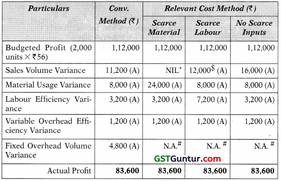
(i) RECONCILE the budgeted and actual profit with the help of variances according to each of the following method:
(A) The conventional method
(B) The relevant cost method assuming that
(a) Materials are scarce and are restricted to supply of 20,000 Kgs. for the period.
(b) Labour hours are limited and available hours are only 16, 000 hours for the period.
(c) There are no scarce inputs. (12 Marks)
(ii) COMMENT on efficiency and responsibility of the Sales Manager for not using scarce resources. (8 Marks) [May 2018 Exam]
Answer:
(I) Computation of Variances
Material Usage Variance = Standard Price × (Standard Quantity – Actual Quantity)
= ₹ 4.00 × (18,000 × Kgs. – 20,000 Kgs.)
= ₹ 8,000(A)
(1,800 units × 20,000 Kgs./2,000 units)
Labour Efficiency = Standard Rate × (Standard Hours – Variance Actual Hours)
= ₹ 8.00 × (14,400 hrs. – 14,800 hrs.)
= ₹ 3,200(A)
*(1,800 units × 16,000 hrs./2,000 units)
Variable Overhead Efficiency Variance = Standard Variable Overheads for Production – Budgeted Variable Over heads for Actual hours
= (14,400 hrs. × ₹ 3.00) – (₹ 3.00 × 14,800 hrs.)
= ₹ 1,200(A)
Fixed Overhead Volume Variance
= Absorbed Fixed Overheads – Budgeted Fixed Overheads
= (14,400 hrs. × ₹ 3.00) – (16,000 hrs. × ₹ 3.00)
= ₹ 4,800(A)
Sales Margin Volume Variance = Standard Margin – Budgeted Margin
= (1,800 units × ₹ 56.00) – (2,000 units × ₹ 56.00)
= ₹ 11,200 (A)
Sales Contribution Volume Variance
= Standard Contribution – Budgeted Contribution
= (1,800 units × ₹ 80.00) – (2,000 units × ₹ 80.00)
= ₹ 16,000 (A)
Statement Showing “Reconciliation Between Budgeted Profit & Actual Profit”

Notes
Scarce Material
Based on conventional method, direct material usage variance is ₹ 8,000 (A) i.e. 2,000 Kg. × ₹ 4. In this situation material is scarce, and, therefore, material cost variance based on relevant cost method should also include contribution lost per unit of material. Excess usage of 2,000 Kg. leads to lost contribution of ₹ 16,000 i.e. 2,000 Kgs. × ₹8. Total material usage variance based on relevant cost method, when material is scarce will be: ₹ 18,000 (A) + ₹ 16,000 (A) = ₹ 24,000 (A). Since labour is not scarce, labour variances are identical to conventional method.

Excess usage of 2,000 Kgs. leads to loss of contribution from 200 units i.e. ₹ 16,000 (200 units × ₹ 80). It is not the function of the sales manager to use material efficiently. Hence, loss of contribution from 200 units should be excluded while computing sales contribution volume variance.
(*) →
Therefore, sales contribution volume variance, when materials are scarce will be NIL i.e. ₹ 16,000 (A) – ₹ 16,000 (A).
Scarce Labour
Material is no longer scarce, and, therefore, the direct material variances are same as in conventional method. In conventional method, excess labour hours used are: 14,400 hrs. – 14,800 hrs. = 400 hrs. Contribution lost per hour = ₹ 10. Therefore, total contribution lost, when labour is scarce will be: 400 hrs. × ₹ 10 = ₹ 4,000. Therefore, total labour efficiency variance, when labour hours are scarce will be ₹ 7,200 (A) i.e. ₹ 3,200 (A) + ₹ 4,000 (A).
Excess usage of 400 hrs. leads to loss of contribution from 50 units i.e. ₹ 4,000 (50 units × ₹ 80). It is not the function of the sales manager to use labour hours efficiently. Hence, loss of contribution from 50 units should be excluded while computing sales contribution volume Variance.
($) →
Therefore, sales contribution volume variance, when labour hours are Scarce will be ₹ 12,000 (A) i.e. ₹ 16,000 (A) – ₹ 4,000 (A).
Fixed Overhead Volume Variance
(#) →
The fixed overhead volume variance does not arise in marginal costing system. In absorption costing system, it represents the value of the under or over absorbed fixed overheads due to change in production volume. When marginal costing is in use there is no overhead volume variance, because marginal costing does not absorb fixed overheads.

(ii) Comment on Efficiency and Responsibility of the Sales Manager
In general, Gross Profit (or contribution margin) is the joint responsibility of sales managers as well as of production managers. On one hand the sales manager is responsible for the sales revenue part, on the other hand the production manager is accountable for the cost- of-goods-sold component. However, it is the top management who needs to ensure that the target profit is achieved by the organization.

The sales manager is accountable for prices, volume, and mix of the product, whereas the production manager must control the costs of materials, labour, factory overheads and quantities of production. The purchase manager must purchase materials at budgeted prices. The personnel manager must employ right people at the right place with appropriate wage rates. The internal audit manager must ensure that the budgetary figures for sales and costs are being adhered by all departments which are directly or indirectly involved in contribution of making profit. Thus, sales manager is not responsible for contribution lost due to excess usage or inefficient usage of resources in case of scarce resources. Hence, such contribution lost must be excluded from the sales contribution volume variance.

Question 22.
(Reconciliation of Budget Profit to Actual Profit through Marginal Costing)
Osaka Manufacturing Co. (OMC) is a leading consumer goods company. The budgeted and actual data of OMC for the year 2020-21 are as follows-

Particulars	Budget	Actual	Variance
Sales/Production (units)	2,00,000	1,65,000	(35,000)
Sales (₹)	21,00,000	16,92,900	(4,07,100)
Less: Variable Costs )	12,66,000	10,74,150	1,91,850
Less: Fixed Costs (t)	3,15,000	3,30,000	(15,000)
Profit	5,19,000	2,88,750	(2,30,250)

The budgeted data shown in the table is based on the assumption that total market size would be 4,00,000 units but it turned out to be
3,75,0 units.
Required
PREPARE a statement showing reconciliation of budget profit toactual profit through marginal costing approach for the year 2020-21 in as much detail as possible.
Answer:
Statement of Reconciliation – Budgeted Vs Actual Profit

Particular	₹
Budgeted Prolit	5,19,00
Less: Sales Volume Contribution – Planning Variance (Adverse)	52,125
Less: Sales Volume Contribution – Operational Variance (Adverse)	93,825
Less: Sales Price Variance (Adverse)	39,600
Less: Variable Cost Variance (Adverse)	29,700
Less: Fixed Cost Variance (Adverse)	15,000
Actual Profit	2,88,750

Workings:
Basic Workings

Calculation of Variances:
Sales Variances:
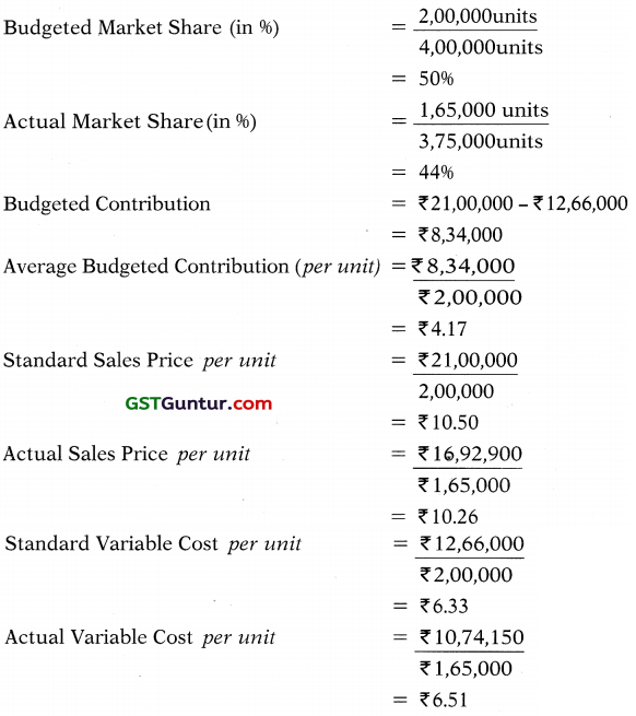
Volume Contribution Planning* = Budgeted Market Share % × (Actual Industry Sales Quantity in units – Budgeted Industry Sales Quantity in units) × (Average Budgeted Contribution per unit)
= 50% × (3,75,000 units – 4,00,000 units) × ₹ 4.17
= 52,125 (A)
(*) Market Size Variance

Volume Contribution Operational** = (Actual Market Share % – Budgeted Market Share %) × (Actual Industry Sales Quantity in units) × (Average Budgeted Contribution per unit)
= (44% – 50 %) × 3,75,000 units × ₹4.17
= 93,825 (A)
(**) Market Share Variance
Price = Actual Sales – Standard Sales
= Actual Sales Quantity × (Actual Price – Standard Price)
= 1,65,000 units × (₹ 10.26 – ₹ 10.50)
= 39,600 (A)

Variable Cost Variances
Cost = Standard Cost for Production – Actual Cost
= Actual Production × (Standard Cost per unit- Actual Cost per unit)
= 1,65,000 units × (₹6.33 – ₹6.51)
= 129.700(A)

Fixed Cost Variances
Expenditure = Budgeted Fixed Cost – Actual Fixed Cost
= ₹ 3,15,000 – ₹ 3,30,000
= ₹ 15,000 (A)

Question 23.
(Investigation of Variances)
NZSC’O Ltd. uses standard costing system for manufacturing its single product ‘ANZ’ Standard Cost Card per unit is as follows:

	(₹)
Direct Materia! (1 kg per unit)	20
Direct Labour (6 hrs @ ₹ 8 per hour)	48
Variable Overheads	24

Actual and Budgeted Activity Levels in units for the month of Feb’21 are:

	Budget	Actual
Production	50,000	52,000

Actual Variable Costs for the month of Feb’ 21 are given as under:

Direct Material	10,65,600
Direct Labour (3,00,000 hrs)	24,42,000
Variable Overheads ,	12,28,000

Required
INTERPRET Direct Labour Rate and Efficiency Variances.
Answer:
INTERPRETATION
Direct Labour Rate Variance:
Adverse Labour Rate Variance indicates that the labour rate per hour paid is more than the set standard. The reason may include among other things such as:
(1) While setting standard, the current/future market conditions like pending labour negotiation/cases, has not been considered (or predicted) correctly.
(2) The labour may have been told that their wage rate will be raised or bonus will be paid if they work efficiently.

Direct Labour Efficiency Variance:
It indicates that the workers has produced actual production quantity in less time than the time allowed. The reason for favourable labour efficiency variance may include among the other things as follows:
(1) While setting standard, workers efficiency could not be estimated properly, this may happen due to non-observance of time and motion study.
(2) The workers may be new in the factory, hence, efficiency could not be predicated properly.
(3) The foreman or personnel manager responsible for labour efficiency, while providing his/her input at the time of budget/standard, has 1 adopted conservative approach.
(4) The increase in the labour rate might have encouraged the labours to do work more efficiently.
In this particular case it may have happened that since labour payment has been increased labour efficiency has also been increased. In a nutshell y because of additional labour rate (Adverse), labour efficiency has gone up §: (Favourable)
Workings
Labour Rate Variance = Standard Cost of Actual Time – Actual Cost
= (SR × AH) – (AR × AH)
Or
= (SR – AR) × AH
= (₹ 8.00 – ₹ 8.14) × 3,00,000 hrs.
= ₹ 42,000 (A)
Working
Actual Labour Rate per hour = $\frac{\text { Actual Paid }}{\text { Actual Hours }}$
= $\frac{₹ 24,42,000}{3,00,000 \mathrm{hrs}}$
= ₹ 8.14
Labour Efficiency Variance = Standard Cost of Standard Time for Actual Production Standard Cost of Actual Time
= (SH × SR) – (AH × SR)
Or
= (SH – AH) × SR
= (3,12,000 hrs. – 3,00,000 hrs.) × ₹ 8.00 = ₹ 96,000 (F)
Working:
Standard Hours = Actual Production × Std. hrs. per unit
= 52,000 units × 6 hrs.
= 3,12,000 hrs.

Question 24.
(Investigation of Variance)
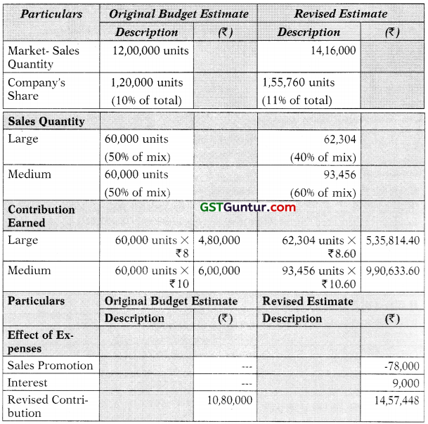
A company is planning to improve its profit level at least by 10% from the preliminary budget estimates of a profit of ₹ 32,80,000 for the coming year. It has worked out the following profit improvement plan:
(i) In the year just concluded the sales of the company were 10% of the total market of 12,00,000 units. For the preparation of the original budget estimate, the same market demand and the same share of market for the company was envisaged. Now it has been estimated that the total market demand will increase by 18 % and the company’s market share will increase to 11% from the present level of 10%.
(ii) The products are sold in two sizes – large and medium. The sales mix of each size was 50:50 so far. Now it is planned that the sales will be 40% of large and 60% of medium. The medium packs and large packs have a contribution of ₹ 10 and ₹ 8 per pack respectively. The budget proposes to raise the price in such a manner that the contribution per pack will increase by ₹ 0.60 for each size.
(iii) There will bean additional expenditure on sales promotion worth ₹ 78,000.
(iv) The company proposes to save ₹ 19,000 by saving on interest cost in the coming year by better financial management.
You are required to draw a profit improvement plan in financial terms and spell out separately the effect of various factors on profit. [May 2018 Exam] (10 Marks)
Answer:
Statement Showing Change in Profit

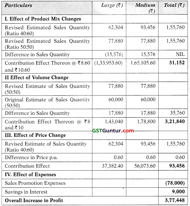
Total Improvement in Profit ₹ 3,77,448 (11.51%).

Workings
Budget for Original and Revised Contribution

Question 25.
(Sales Variance)
T-tech is a Taiwan based firm, that designs, develops, and sells audio equipment. Founded in 1975 by Mr. Boss, firm sells its products throughout the world. T-tech is best known for its home audio systems and speakers, noise cancelling headphones, professional audio systems and automobile sound system. Extracts from the budget are shown in ; the following table:
Home Audio System Division Jan ’ 2021

System	Sales (units)	Selling Price (₹)	Standard Cost (per System) (₹)
3.000 WPMPO	1,500	18,750	12,500
5,000 WPMPO	500	50,000	26,250

The Managing Director has sent you a copy of an email he received from the Sales Manager ‘K’. The content of the email was as follows:
“We have had an outstanding month. There was an adverse Sales Price Variance on the 3,000 W PMPO Systems of ₹ 22,50,000 but I compensated for that by raising the price of 5,000 W PMPO Systems. Unit sales of 3,000 WPMPO Systems were as expected but sales of the 5,000 W PMPOs were exceptional and gave a Sales Margin Volume Variance of 23,75,000.1 think I deserve a bonus!”
The managing Director has asked for your opinion on these figures. You got the following information.
Actual results for Jan’ 2021 were:

System	Sales (unit)	Selling Price ₹
3,000 W PMPO	1,500	17,250
5,000 W PMPO	600	53,750

The total market demand for 3,000 WPMPO Systems was as budgeted but as a result of suppliers reducing the price of supporting UHD TV System the total market for 5,000 WPMPO Systems raised by 50% in Jan’2021.
The company had sufficient capacity tomeet the revised market demand for 750 units of its 5,000 WPMPO Systems and therefore maintained its market share
Requited
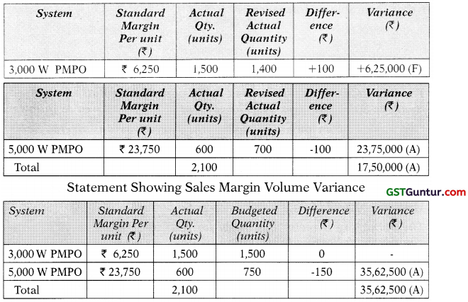
(i) CALCULATE the following Operational Variances based on the revised market details:
– Sales Margin Mix Variance
– Sales Margin Volume Variance. (4 marks)
(ii) COMMENT briefly on the measurement of the K’s performance. (6 marks) [May 2018 RTP]
Answer:
(i) Statement Showing Sales Margin Mix Variance:

(ii) A Planning Variance simply compares a revised standard (that should or would have been use if planners had known in advances what was going to happen) to the original standard. A planning variance is considered as not to be controllable by management.
The market size is not within the control of the sales manager and therefore variances caused by changes in the market size would be regarded as planning variances.
However, variances caused by changes in the selling price and consequently the selling price variances and market shares would be within the control of the sales manager and treated as operating variances.

The market size variance compares the original and revised market sizes. This is unchanged for 3,000 W PMPO Systems so the only variance that occurs relates to the 5,000 W PMPO Systems and is ₹ 59,37,500 (F) [250 system × ₹23,750].
It is vital to make this distinction because as can be seen from the scenario the measurement of the “K”s performance is incomplete if the revised market size is ignored.
The favourable volume variance of ₹ 23,75,000 referred to in the “K”s e-mail is made up of two elements, one of which, the market size, is a planning variance which is outside his control. It is this that has caused the overall volume variance to be favourable, and thus ‘K’ is not responsible for the overall favorable performance.

Question 26.
(Investigation of Variances)
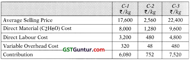
Queensland Chemicals (QC) manufactures high-quality chemicals C-1, C-2 and C-3. Extracts from the budget for last year are given below:

	C-l	C-2	C-3
Sales Quantity (kg)	1,000	3,250	750
	₹/kg	₹/kg	₹/kg
Average Selling Price	17,600	2,560	22,400
Direct Material (Cflfl) Cost	8,000	1,280	9,600
Direct Labour Cost	3,200	480	4,800
Variable Overhead Cost	320	48	480

The budgeted direct labour cost per hour was ₹ 160.
Actual results for last year were as follows:

	C-l	C-2	C-3
Sales Quantity (units)	900	3,875	975
	₹/kg	₹/kg	₹/kg
Average Selling Price	19,200	2,480	20,000
Direct Material (C₂H₆O) Cost	8,800	1,200	10,400
Direct Labour Cost	3,600	480	4,800
Variable Overhead Cost	480	64	640

The actual direct labour cost per hour was ₹ 150. Actual variable overhead cost per direct labour hour was ? 20. QC follows just in time system for purchasing and production and does not hold any inventory.
Required
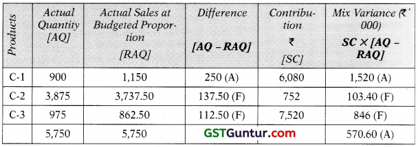
INTERPRET the Sales Mix Variance and Sales Quantity variance in terms of contribution. (10 Marks) [Aug. 2018 MTP]
Answer:
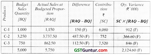
Variance Interpretation
The sales quantity variance and the sales mix variance describe how the sales volume contribution variance has been affected by a change in the total quantity of sales and a change in the relative mix of products sold.

From the figures arrived for the sales quantity contribution variance, we can observe that the increase in total quantity sold would have gained an additional contribution of ₹ 2,124,600, if the actual sales volume had been in the budgeted sales proportion.

The sales mix contribution variance shows that the variation in the sales mix resulted in a curtailment in profit by 5,70,600. The change in the sales mix has resulted in a relatively higher proportion of sales of C-2 which is the chemical that earns the lowest contribution and a lower proportion of C-1 which earn a contribution significantly higher. The relative increase in the sale of C-3 however, which has the highest unit contribution, has partially offset the switch in mix to C-2.

Workings
Statement Showing Standard Contribution

Sales Contribution Mix Variance

Sales Contribution Quantity Variance

Question 27.
(Total Variance)
Apple Ltd., is following three variances method to analyse and un-derstand production overhead variances. The three variances for a particular year were reported as given below:

Production overhead expenditure variance	94,000 A
Production overhead volume variance	1,00,000 F
Production overhead efficiency variance	48,000 F

The other particulars furnished from the records of the company are:

Standard machine hours for the year	11,500
Closing balance in the Production Overhead Control Account	₹ 18,00,000
Fixed overhead rate per hour	₹ 125
Variable overhead rate per hour	₹ 80

Required:
COMPUTE the following by considering the additional information also:
(i) Actual machine hours
(ii) Budgeted machine hours
(iii) Total Fixed Production Overhead amount
(iv) Applied Production Overhead amount (10 Marks)
Additional Information

Expenditure variance was computed totally for fixed and variable overheads.
Volume variance is applicable to fixed overhead only.
Efficiency variance is applicable only to variable overhead and fixed overhead efficiency variance was already included in volume variance. [Nov. 2018 Exam]

Answer:
(i) Calculation of Actual Machine Hours
Efficiency Variance = ₹ 48,000 (F) given
= Standard Variable Overhead Rate per Hour (Standard Hours – Actual Hours)
₹ 48,000(F) = ₹ 80 × (11,500 hrs. – Actual Hours)
Actual Hours = 10,900 hrs.

(ii) Budgeted Machine Hours
Volume Variance = ₹ 1,00,000 (F)
= Standard Fixed Overhead Rate per × Hour (Standard Hours – Budgeted Hours)
₹ 1,00,000 (F) = ₹ 125 × (11, 500 hrs. – Budgeted Hours)
Budgeted Hours = 10,700 hrs.
Total Fixed Production Overhead*
Fixed Production Overhead = Standard Fixed Overhead Rate per Hour × Budgeted Hours
= ₹ 125 × 10, 700 hrs.
= ₹ 13.37,500
* Assumed Budgeted
Applied Manufacturing Overhead
= Standard Overhead Rate per Hour × Standard Hours
= ₹ 205 × 11, 500 hrs.
= ₹ 23,57,500
ALTERNATIVES (iii) & (iv)

(iii) Total Fixed Production Overhead
Expenditure Variance = Fixed Production Overhead(Budgeted) + Budgeted Variable Overheads for Actual Hours – Actual Overheads ₹ 94,000 (A) = Fixed Production Overhead + 10,900 hrs. × ₹ 80 – ₹ 18,00,000
Fixed Production Overhead – ₹ 8,34,000

(iv) Applied Manufacturing Overhead
= Actual Overhead Incurred + Total Variance
= ₹ 18,00,000 + ₹ 54,000
= ₹ 18,54,000

Working Notes
Total Variance = Expenditure Variance + Efficiency Variance + Volume Variance
= ₹ 94,000 (A) + ₹ 48,000 (F) + ₹ 1,00,000 (F)
= ₹ 54,000 (F)

Question 28.
Case Study (Control Through Standard Costing System)
‘HAL’ is a manufacturer, retailer, and installer of Cassette Type Split AC for industrial buyers. It started business in 2001 and its market segment has been low to medium level groups. Until recently, its business model has been based on selling high volumes of a standard AC, brand name ‘Summer’, with a very limited degree of customer choice, at low profit margins. ‘HAL’s current control system is focused exclusively on the efficiency of its manufacturing process and it reports monthly on the following variances: material price, material usage and manufacturing labour efficiency. ‘HAL’ uses standard costing for its manufacturing operations. In 2018, HAL’ employs 20 teams, each of which is required to install one of its ‘Summer’ AC per day for 350 days a year. The average revenue per ‘Summer’ AC installed is ₹ 36,000. ‘HAL’ would like to maintain this side of its business at the current level. The ‘Summer’ installation teams are paid a basic wage which is supplemented by a bonus for every AC they install over the yearly target of 350. The teams make their own arrangements for each installation and some teams work seven days a week, and up to 12 hours a day, to increase their earnings. ‘HAL’ usually receives one minor complaint each time a ‘Summer’ AC is installed and a major complaint for 10% of the ‘Summer’ AC installations.

In 2016, HAL’ had launched a new AC, brand name ‘Summer-Cool’. This AC is aimed at high level corporates and it offers a very large degree of choice for the customer and the use of the highest standards of materials, appliances, and installation. ‘HAL’ would like to grow this side of its business. A ‘Summer-Cool’ AC retails for a minimum of ₹ 1,00,000 to a maximum of X₹ 5,00,000. The retail price includes installation. In 2017 the average revenue for each ‘Summer-Cool’ AC installed was ₹ 3,00,000. Currently, ‘HAL’has 7 teams of ‘Summer-Cool’ AC installers and they can install up to 240 AC a year per team. These teams are paid salaries without a bonus element. ‘HAL’ has never received a complaint about a ‘Summer-Cool’ AC installation.

HAL’s business is generated from repeat orders, recommendations, and local press advertising. It employs three sales executives who earn an annual salary of ₹ 3,00,000 each. It offers a six-month money back guarantee and this has to be fulfilled for l%of its installations. HAL’ has always been in profits but was shocked to see that in its results in 2017 it only earned 0.2% net profit on its turnover.
Required
(i) EVALUATE the appropriateness of ‘HAL’s current control system, (8 Marks)
(ii) RECOMMEND four Critical Success Factors (CSFs) which could assist ‘HAL’ in achieving future success. (8 Marks)
(iii) ADVISE ‘HAL’ about the changes it could implement in its standard costing and reporting system to achieve improved control. (4 Marks) [Nov. 2018 RTPJ
Answer:
(i) HAL’s Control System HAL’s current control system is ‘focusedexclu- sively’ on the manufacturing process and its efficiency even though HAL is also a retailer and installer of industrial ACs. It is suitable for HAL’s control system to monitor manufacturing efficiency with the help of the three variances: material usage, material price and manufacturing labour efficiency. No reasons have been given for 4 focusing on these three variances and there may be other variances which can provide useful control information that are not currently
computed for example, labour rate and material yield. Although HAL uses standard costing, it is unclear whether it calculates product costs. A lack of product costs computation may be the reason that it was shocked about its 2017 profit margin. Standard costing could be in criticism for misdirecting management’s attention. Thus, in the case of a ‘Summer- Cool’ AC where the highest standards of materials are used, it is pertinent that the quality of the finished product is not compromised. Therefore, it might be proper to accept an unfavourable material price variance to maintain the product’s standards. Variance analysis should not be done in isolation but a holistic view needs to be taken about HAL’s operations and the current control system may not lead to this. HAL is not currently controlling and monitoring aspects which are important for competitive success.

HAL’s Critical Success Factors have not been identified yet. There is monthly reporting of variances but in addition to this, there should also be follow-up actions for outcome resulting from these reports. However, a month is not inevitably the relevant reporting period for all aspects of HAL’s business. If there is a production problem leading to excessive materials wastages, a month is too long time to wait before remedial action are taken. Therefore, real-time or coexistent reporting may be more relevant for manufacturing operations. A major deficiency of HAL’s control systems is that they do not extend to retailing and installation activities. The ‘Summer’ installation teams are incentivized to complete ACs which could be good for their productivity. However, there is a high level of complaints associated with their work. As there is no evident means of the installation team’s work, the reasons of the complaints cannot be identified.

(ii) Critical Success Factors (CSF) are elements tied to the strategy of business and they represent objectives that business is trying to achieve, as a corporation, as a department or as a business unit, Critical success factors may vary over time and may include items like employee attitudes, manufacturing flexibility etc. There are a range of CSF’s which could be appropriate for HAL. They include: CSF: Installations Quality There are different quality expectations for the two ACs and there have been different levels of quality achieved, can be seen in the historic pattern of complaints. This strongly implies that the quality of installation should be tracked as a separate CSF for each AC. This CSF is important for HAL due to cost implications of rectifications and guarantee claims. It is also important to consider that because of the effect that poor quality will have on HAL’s future business.

CSF: Customer Satisfaction Like quality, this CSF will need to be monitored separately for each AC. Customer satisfaction encompass the complete life of a transaction beginning with the initial enquiry about a purchase and continuing after installation for the life of the AC. Customer satisfaction will have an influence on HAL’s future ; business which is dependent, in part, on repeat orders and recommendations. This CSF will also show the market’s view of HAL’s brand.

CSF: Brand Performance HAL has two distinct brands. They are directed at different market segments and have different associated attributes. ‘Summer’ ACs offer limited choice to the customer and : retail, on average, for ₹ 36,000. HAL would like to maintain this business at its present level (7,000 ACs a year minimum) ₹ 252 million revenue. HAL needs to ascertain where this brand is situated in its life-cycle and what marketing activities may be required to support it. The ‘Summer-Cool’ brand is aimed at a different market segment and HAL would like to grow this aspect of its business which produces revenue of ₹ 504 million. The success of both brands is important for the continual success of HAL and this CSF indicate a complete view of performance.

CSF: Manufacturing Excellence HAL manufactures all the ACs which ! it sells and installs. Manufacturing must be a substantial part of HAL’s total costs and a significant contributor to profitability. Currently, HAL monitors some limited aspects of manufacturing through its control system. However, there are many other aspects which have not been reported upon, for example- innovation, labour absentism, manufacturing flexibility and investment in technology. This CSF is much broader than the current control system. It also assists in searching for competitiveness.

(iii) Standard Costing and Reporting System HAL may be required to abandon or modify its standard costing and reporting system. The rationale behind this is that the current control system might lead to an inappropriate emphasis being placed on certain aspects of performance. It is noteworthy that the installations for ‘Summer’ AC is causing a substantial level of complaints whereas there has never been a complaint made about a ‘Summer Cool’ AC. It could be that the different remuneration arrangements for the ACs’ installation teams have led to this and as the complaint level is an important aspect of the CSF ie. Customer Satisfaction, HAL may need to modify its remuneration arrangements.

It should also reckon whether it would be benefited from a broader range of variance reporting, for example, it may find reporting useful to report on labour rates and material yield. For all CSFs, HAL will need to determine the appropriate reporting intervals. Although it is useful to synchronize this with the accounting reporting cycle, CSFs and KPIs do not necessarily coexist with accounting period ends. Some KPI’s may require to be reported in real-time, for example, material wastage, others may be of a longer duration like Customer Satisfaction. There is a strong argument for disassociation of the CSFs reporting from the financial reporting cycles.

Question 29.
(Reconciliation, Investigation of Variance)
Established in the year 1999, Fast Food Company is the pioneer of fast food in Southampton. It delivers a truly fresh, affordable, made to order sandwiches, burger, and other meal in a friendly and relaxed environment. The popularity of the sandwiches, burger etc. continued to grow over the decades but one thing remained the same and that was its core values and principles:

Always provide exceptional service to valued guests;
Provide the highest quality menu items at a price everyone can afford and enjoy; and
Keep operating costs low and ensure to have great systems in place and never stop improving.

It provides a comfortable place for people to unwind over interesting conversations. From the beginning, as it continues to grow, it is guided by passion for delighting customers by serving fresh, delicious food right in front of customer.
The performance report* for FY 2018-19 was presented at the management committee meeting as follows:

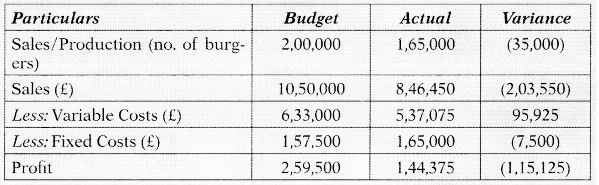
* burger segment
The Management Accountant of FF believed that the size of the fast-food market deriving the budget number of burgers to be sold is over-estimated. He has computed the value of the sales volume contribution planning variance to be 26,062.50 adverse. 2
Further, the report also included customer’s feedback and the majority £ of comments were regarding delay in service time. One of feedback was as follows:

“I ordered two burgers at 2:10 pm. After half an hour (30 minutes) j of waiting I called the waiter and asked him what happened? he told me that he will check with kitchen. I got the order after 45 minutes of waiting, this cafe is not good in delivery time”
The budgeted data shown in the table is based on the assumption that total market size would be 4,00,000 units.
Required
(i) PREPARE a reconciliation statement of budgeted profit to actual profit through marginal costing approach in as much ) detail as possible.
(ii) EXPLAIN the implications of the reconciliation statement.
(iii) Management is worried about customer’s feedback. ADVISE measures to improve delivery service time. [Nov. 2019 R.TP]
Answer:
(i) Statement of Reconcilliation – Budgeted Vs Actual Profit

Particulars	£
Budgeted Profit	2,59,500
Less: Sales Volume Contribution – Planning Variance (Adverse)	26,062.50
Less: Sales Volume Contribution – Operational Variance (Adverse)	46,912.50
Less: Sales Price Variance (Adverse)	19,800
Less: Variable Cost Variance (Adverse)	14,850
Less: Fixed Cost Variance (Adverse)	7,500
Actual Profit	1,44,375

Workings:
Basic Workings
Budgeted Market Share (in %) = $\frac{2,00,000 \text { units }}{4,00,000 \text { units }}$
= 50%
Budgeted Contribution = £10,50,000 – £6,33,000 = £4,17,000
Average Budgeted Contribution (per unit)

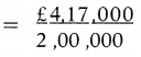
= £2.085
Volume Contribution Planning = Budgeted Market Share % × (Actual Industry Sales Quantity in units – Budgeted Industry Sales Quantity in units) × (Average Budgeted Contribution per unit)
⇒ £26,062.50 (A) = 50% × (Actual Industry Sales Quantity in units – 4,00,000 units) × £2.085
⇒ Actual Industry Sales Quantity = 3,75,000 units
⇒ Actual Market Share (in %) = $\frac{1,65,000 \text { units }}{3,75,000 \text { units }}$ £3.255
= 44%
Standard Sales Price per unit = $\frac{£ 10,50,000}{2,00,000}$
= £5.25
Actual Sales Price per unit = $\frac{£ 8,46,450}{1,65,000}$
= £5.13
Standard Variable Cost per unit = $\frac{£ 6,33,000}{2,00,000}$
= £3.165
Actual Variable Cost per unit = $\frac{£ 5,37,075}{1,65,000}$
= £3.255

Calculation of Variances
Sales Variances
Volume Contribution Operational = (Actual Market Share % – Budgeted Market Share %) × (Actual Industry Sales Quantity in units) × (Average Budgeted Contribution per unit)
= (44% – 50 %) × 3,75,000 units × £2.085
= £46,912.50 (A)
Price = Actual Sales – Standard Sales
= Actual Sales Quantity × (Actual Price – Standard Price)
= 1,65,0 units × (£5.13 – £5.25)
= £19,800 (A)

Variable Cost Variances
cost = Standard Cost for Production – Actual Cost
= Actual Production × (Standard Cost per unit – Actual Cost per unit)
= 1,65,000 units × (£3.165 – £3.255)
= £14,850 (A)

Fixed Cost Variances
Expenditure = Budgeted Fixed Cost – Actual Fixed Cost
= £1.57,500 – £1,65,000
= £7,500 (A)

(ii) Implications of Reconciliation Statement
In the revised statement, the sales volume variance has been detailed by the way of two variances i.e. planning and operational variances. This kind of detailed information assists the company to check, which kind of variances are under the management control and which are not. FF has adverse volume contribution planning variance and the reason of could be the environmental/ market changes, that was not anticipated at the time of budget preparation, so they are not under management control and hence, no one is responsible for this. On the other hand, the sales volume contribution operational variance was under control of the managers and they should be held responsible for the same. The reason of adverse sales volume contribution operational variance could be unsuccessful direct selling efforts/marketing efforts. FF has adverse sales price variance as well. It indicates that the burgers were sold for lower price than standard. The reason of this could be unforeseen market competitive price, tapping new’ market etc.

Further, revised reconciliation statement delivers little information about the variable cost and fixed cost variances. They both are adverse. Fixed cost consists of many items such as salaries, annual maintenance cost, rent and insurance etc. Often fixed cost items are not affected in short run in response to change in the level of activity, but they might change in response to other factors such as price. This may cause increase expenditure on fixed overheads. A meaningful analysis of fixed cost variance requires a line to line comparison of budgeted cost with actual cost.

In case of FF, the variable cost may be made up of large individual different items such as vegetables, gas, indirect labour, regular maintenance cost etc. Control of variable cost also requires line by line analysis for each individual item. The adverse variable cost variance simply reveals that FF incurred more on variable cost than expected. However, it is necessary to take into consideration the causes of this adverse variance which is beyond the control of the management, for instance, the unusual price hike in vegetables in case of unseasonal rainfall.

(iii) Measures to Improve Fast Food Delivery Service Time
Customers expect that their food order to be delivered quickly. From customer’s feedback in the question, it is evident that FF has a problem in food delivery, due to which, customers go unsatisfied. The reason of late delivery could be non- availability of raw material on time or employees not working properly etc. The reason of employees not working properly could be job dissatisfaction which may be due to improper working conditions, low salary, or no reward for overtime etc.

In order to reduce delivery time, raw material should be made available in stock based on daily requirement. FF may follow quantitative approach to inventory problems, which lays down clear guidelines that when to re-order or alert the management in exceptional situations.
In addition, FF must also address the issues related to employee and involve them in a loop. FF could improve the employee satisfaction with proper working conditions, better pay, training, and growth opportunities.
Moreover, it is important that customers should be informed about approximate delivery time since this will reduce customer’s anxiety and will proactively reduce any complaints over long waits for delivery of food. If unexpected delays occur, it is important to communicate with customers, apologies for the delay and inform them about the new approximate delivery time along with valid reason.
In addition to this, FF can also introduce pagers or install electronic board displaying ticket number or seif-serve kiosks allowing customers to roam around or order in advance so that they do not have long waiting time.

Question 30.
Case Scenario (Interpretation of Variance)
Natural Spices manufactures and distributes high-quality spices to gourmet food shops and top quality restaurants. Gourmet and high- end restaurants pride themselves on using the freshest, highest-quality ingredients.
Natural Spices has set up five state of the art plants for meeting the ever- growing demand. The firm procures raw material directly from the centers of produce to maintain uniform taste and quality. The raw material is first cleaned, dried and tested with the help of special machines. It is then carefully grounded into the finished product passing through various stages and packaged at the firm’s ultraclean factory before being dispatched to customers.
The following variances pertain to last week of operations, arose as a consequence of management’s decision to lower prices to increase volume.

Sales Volume Variance	18,000 (F)
Sales Price Variance	14,000 (A)
Purchase Price Variance	10,000 (F)
Labour Efficiency Variance	11,200 (F)
Fixed Cost Expenditure Variance	4,400 (F)

Required
(i) IDENTIFY the‘Critical Success Factors’for Natural Spices,
(ii) EVALUATE the management’s decision with the ‘Overall Corporate Strategy’ and ‘Critical Success Factors’.
Answer:
(i) Gourmet and high-end restaurants recognises Natural Spices on the basis of its high quality of spices. Therefore, quality is most critical success factor of Natural Spices. There are other factors which cannot be ignore such as price, delivery options, attractive packing etc. But all are secondary to the quality.

(ii) Deliberate action of cutting price to increase sales volume indicates that firm is intending to expand its market to retail market and street shops which is price sensitive.
Purchase Price Variance is clearly indicating that firm has purchased raw material at lower price which may be due to buying of lower quality of material. Similarly, positive Efficiency Variance is indicating cost cutting and stretching resources.

It appears that firm is intending to expand its market to retail market and street shops by not only reducing the price but also compromising its quality which is opposing its current strategy of high quality.
Management should monitor the trends of variances on regular basis and take appropriate action in case of evidence of permanent decline in quality. Here, customer feedback is also very important.

Question 31.
(Investigation of Variance)
Aquatic Feed (AF) is the leading manufacturer of fish and other sea animal feed. AF has made its credit pioneering effort and service for over one decade in development of culture, processing and exports with its state-of-art fish feed and processing plants. Hallmark of AF is constant upgradation of aquaculture technology bringing latest developments in the field to the doorstep of the Indian aquaculture farmer. It stands-as a leading provider of high quality feed, best technical support to the farmer and caters to the quality standards of global customers.
One of its fish feed product is “B” which is produced by mixing and heating three ingredients: B1, B2 and B3. It uses a standard costing system to monitor its costs.
The standard material cost for 100 Kg. of “B” is as follows:

Ingredients	Standard Qty. (Kg)	Cost per Kg. (₹)	Cost per 100 Kg. of “B” (₹)
B1	42	3	126
B2	62	6	372
B3	21	2	42
	125		540

Notes:
+ B1, B2 and B3 are agricultural products. Their quality and price change significantly every year. Standard prices are determined at the average market price over the last three years. AF has a purchasing manager responsible for purchasing and pricing.

The standard mix is decided by the Managing Partner having 15 years’ rich experience in aquaculture field. The last time this was done at time of launching the “B” that was six years back. The standard mix has not been changed since.
Mixing and heating process are subject to some evaporation loss.

In current month 4,605 Kg. of “B” was produced, using the following ingredients:

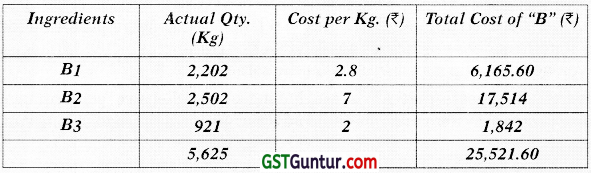
At every month end, the production manager receives a statement from the Managing Partner. This statement contains material price and usage variances for the month and no other feedback on the efficiency of the processes is provided.
Required
EVALUATE the performance measurement system in AF.
Answer:
The statement reported, ₹ 2,062 favourable material price variance. The responsibility for controlling the materials price variance is usually the purchasing manager’s. Undoubtedly, in current scenario, the price of materials is largely beyond his or her control; however, the price variance can be influenced by such factors as quality, quantity discounts, distance of supplier’s location, and so on. These factors are often under the control of the purchase manager. The production manager is responsible for material usage and cannot be held responsible for the material price variance.

Since total usage variance reported, ₹ 1,406 favourable, production manager could assume good performance. However, if usage variance is considered in more detail, through the mix and yield calculations, it can be observed that variance was driven by a change in the mix and by using a mix of ingredients which was different from standard, it has resulted in a saving of ₹ 840; Similarly, it has led to a favourable yield. It is worthwhile to note that changing the mix could impact the product quality and sales as well, however, no information has been given about this.

Prices and quality of three agriculture ingredients are changing significantly every year. Using ex ante prices and usage standards can implicit an outdated view of variances. Failing to separate variances caused by uncontrollable factors and planning errors from variances caused by controllable factors can be demoralizing for the managers.

In addition, managers are not involved in setting the standard mix and the same has not been changed for six years despite continuous changes in the quality and prices of the ingredients. This can also mislead the managers i.e. to carryout control activities which are based on the outdated standards.

Furthermore, a true image is missing in relation to managers’ performance as statement does not include any feedback or comments on the variances. Even no follow up is being taken on the same.
Overall, it appears that AF is not having comprehensive performance measurement system and this could adversely impact the firm in long run.
Working:

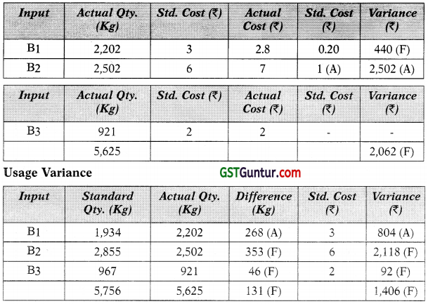
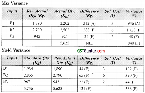
Question 32.
(Variance Analysis)
YLtd., based in Kuala Lumpur, is the Malaysian subsidiary of Japan’s NY corporation, headquartered in Tokyo. Y’s principal Malaysian businesses include marketing, sales, and after – sales sendee of electronic products & software exports products. Y set up a new factory in Penang to manufacture and sell integrated circuit ‘Q50X-N’. The first quarter’s budgeted production and sales were 2,000 units. The budgeted sales price and standard costs for ‘Q50X-N ’ were as follows:

	RM	RM
Standard Sales Price per unit		50
Standard Costs per unit
Circuit X (10 units @ RM 2.5)	25
Circuit Designers (6 hrs. @ RM 2)	12	(37)
Standard Contribution per unit		13

Actual results for the first quarter were as follows:

	RM ’000	RM’000
Sales (2,000 units)		158
Production Costs (2,000 units)
Circuit × (21,600 units)	97.20
Circuit Designers (11,600 hours)	34.80	(132)
Actual Contribution (2,000 units)		26

The management accountant made the following observations on the actual results-
“In total, the performance agreed with budget; however, in every aspect other than volume, there were huge differences. Sales were made at what was supposed to be the highest feasible price, but we now feel that we could have sold for RM82.50 with no adverse effect on volume. The Circuit X cost that was anticipated at the time the budget was prepared was RM 2.5 per unit. However, the general market price relating to efficient purchases of the Circuit X during the quarter was RM 4.25 per unit. Circuit designers have the responsibility of designing electronic circuits that make up electrical systems. Circuit Designer’s costs rose dramatically with increased demand for the specialist skills required to produce the ‘Q50X-N’, and the general market rate was RM 3.125 per hour – although Y always paid below the normal market rate whenever possible. In my opinion, it is not necessary to measure the first quarter’s performance through variance analysis. Further, our operations are fully efficient as the final contribution is equal to the original budget.”
Required
COMMENT on management accountant’s view. (10 Marks) [Oct. 2020 MTP]
Answer:
Comment:
As the management accountant states, and the analysis (W.N. 1) presents, the overall variance for the Y is nil. The cumulative adverse variances exactly offset the favourable variances i.e. sales price variance and circuit designer’s efficiency variance. However, this traditional analysis does not clearly show the efficiency with which the Y operated during the quarter, as it is difficult to say whether some of the variances arose from the use of incorrect standards, or whether they were due to efficient or inefficient application of those standards.

In order to determine this, a revised ex post plan should be required, setting out the standards that, with hindsight, should have been in operation during the quarter. These revised ex post standards are presented in W.N. 2.
As seen from W.N. 3, on the cost side, the circuit designer’s rate variance has changed from adverse to favourable, and the price variance for component X, while remaining adverse, is significantly reduced in comparison to that calculated under the traditional analysis (W.N.l); on the sales side, sales price variance, which was particularly large „ and favourable in the traditional analysis (W.N.l), is changed into an g adverse variance in the revised approach, reflecting the fact that the Y failed to sell at prices that were actually available in the market.

Further, variances arose from changes in factors external to the business (W.N. 4), which might not have been known or acknowledged by standard-setters at the time of planning are beyond the control of the operational managers. The distinction between variances is necessary to gain a realistic measure of operational efficiency.
W.N.l Y
Quarter-1
Operating Statement

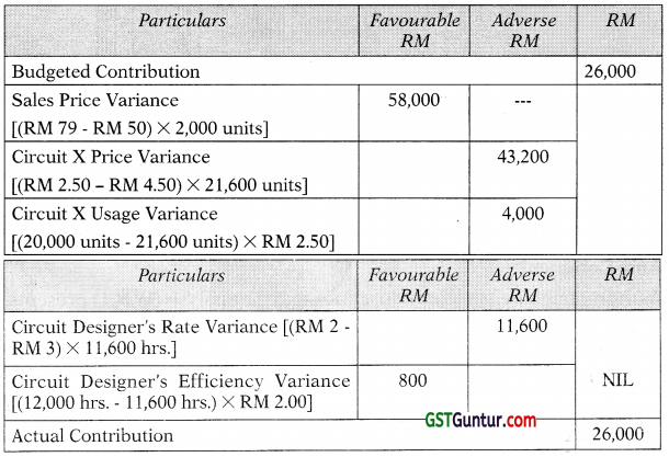
W.NT. 2
Statement Showing Original Standards, Revised Standards, and Actual Results for Quarter 1

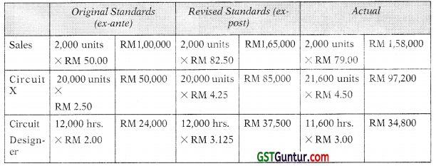
W.N. 3
Statement Showing Operational Variances

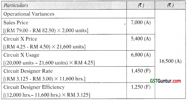
W.N. 4
Statement Showing Planning Variances

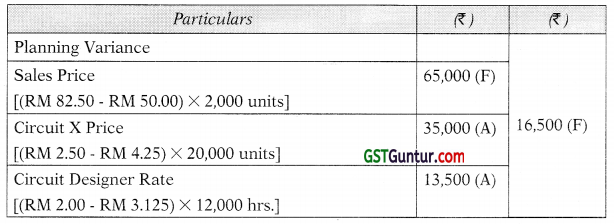
Question 33.
(Variance Analysis)
ZMInc. is a family un business based in Country Z. It is a manufacturer of two types of flooring rolls, one for industrial usage and the other for domestic residential use, throughout mainland of Country Z. The company started with the production of residential domestic flooring. It is now an established player in this market. In the recent years, the company pioneered into making flooring rolls for industrial usage. The management has the following information about the budgeted and actual data for 2020.

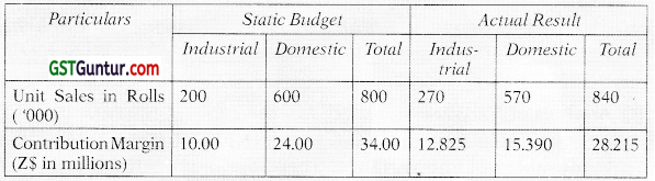
In late 2019, a marketing research estimated market volume for industrial and domestic flooring at 8 m Rolls. Actual market volume for 2020 was 7 m Rolls. Actual sales trend of ZM Inc. is indicative of the sales trends for individual products in the future years, it is likely that they might continue to sell a similar sales trajectory.
A newly appointed accountant has computed following variances from the above data:

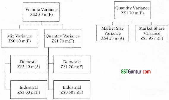
‘m ’ refers to million; assume figures in this chart are correct.
Required
Assuming yourself as a performance management expert of ZM, the CEO has asked you to:
(i) ANALYSE the variances computed by the accountant;
(ii) ADVISE strategic inputs on ‘two types of flooring rolls’ to help out her in strategic decision making. [Nov. 2020 RTP]
Answer:
(i) Analysis of Variances
It can be seen that total unit sales increased by 40,000 rolls resulted in a favourable volume variance. Therefore, a potential increase of Z$2.3 m in contribution margin was achieved as a result of change in sales volume compared with budgeted volume. The volume variance is further divided into a mix and quantity variance. In the case of ZM, mix variance came out to be Z$0.60 m favourable and the quantity variance came out to be favourable Z$ 1.70 m. Favourable mix variance Z$0.60 m indicates that the sales mix shifts toward the industrial flooring rolls ie. high contribution product. ZM sold 40,000 more rolls than were budgeted, resulting in Z$1.70 m favourable quantity variance. Therefore, it is necessary to identify the reasons behind the increase in sales. The reasons may be competitor’s distribution issues, better customer services, or growth in overall market. Further insight into reasons of quantity variance can be gain by analyzing market share and size variances. ZM gain 2 market share percentage points from 10% budgeted share to the actual share of 12%. The Z$5.95 m favourable market share variance may be the effect of the decline in contribution margin rate.

The impact of changing market size on contribution margin can be traced through market size variance. Market size variance is Z$4.25 m adverse as actual market size decreased 12.5% compared to budgeted market size. Further, it appears that accountant has missed to compute the price variance which is a substantial part of the analysis. If we look closely at the data given, the price variance for domestic as well as industrial roll can be computed without difficulty. The price variance for domestic flooring rolls as well as industrial flooring rolls is unfavourable; this indicates that the both varieties were sold a lower margin than standard. This throughout analysis shows a negative impact of Z$ 5.785 m on contribution margin for which price variance is the main contributor. Revised structures after the computation of price variance are as under:

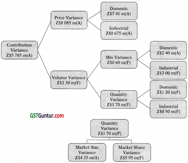
Workings
Contribution Price Variance

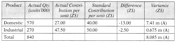
(ii) Strategic Inputs
The actual sale of industrial flooring rolls is 35% higher than projections. However, actual contribution margin of Z$47.5 is marginally lower than standard contribution margin of Z$50 per unit. This indicates that ZM may have cut its selling price to maintain or gain market share. Therefore, industrial flooring rolls are in the Growth

Phase of product life cycle. Due to increase in demand, there is a possibility of higher sales and profits to be made in future years. Similarly, the actual sale of domestic flooring roll is 5% lower than the expectations. However, actual contribution margin is Z$27 per roll i.e. 32.5% lower than the standard contribution margin. This indicates that ZM may have sold these at substantially reduced price to maintain the sales volume. Therefore, the domestic residential flooring rolls might be in the Decline Stage of product life cycle.

The market size for flooring rolls has reduced from an expectation of 80 lacs rolls to 70 lacs rolls. Therefore, the market size has shrunk significantly by 12.5% for the year 2019. This is a threat to profitability of business. The management has to understand the reasons behind this shrinkage. For example, dwindling demand maybe on account of cheaper substitutes available for flooring rolls. The management has to take cognizance of this threat to business. A positive for ZM is that its actual market share for flooring rolls was higher than expected at 12%. An increase in market share would have a beneficial impact on the company’s profitability. Also, despite the shrinkage in market size, demand for industrial flooring rolls seems to be on the rise. This could | be an opportunity for the management to consider.

As explained above, the industrial flooring rolls seem to be in the Growth Stage of product life cycle, while the domestic residential rolls are in the Decline Stage. Industrial flooring rolls have a higher contribution margin per roll as compared to domestic residential rolls. Accordingly, ZMmav consider phasing out domestic flooring rolls and concentrate on industrial flooring rolls. In view of shrinking market conditions, it would be more profitable to phase out the weaker product and concentrate on the fast moving and profitable product. At the same time, since domestic flooring roll still has significant demand, the strategy to phase out this product may have to be done in a phased and well-planned manner. In view of the shrinking market size, ZM should not end up losing its market share due to phasing out domestic flooring rolls.

For Your Conceptual Understanding
“Budgeted Vs Actual Figures”

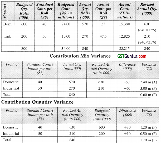
Market Size Variance
= Budgeted Market Share % × ( Actual Industry Sales Quantity in units – Budgeted Industry Sales Quantity in units) × (Average Budgeted Contribution per unit)
= 10% × (70,00,000 Rolls – 80,00,000 Rolls) × ZS 42.50
= Z$ 4.25 m (A)

Market Share Variance
= (Actual Market Share % – Budgeted Market Share %) × (Actual Industry Sales Quantity in units) × (Average Budgeted Contribution per unit)
= (12% – 10%) × 70,00,000 Rolls × Z$ 42.50
= Z$ 5.95 m (F)

Question 34.
Case Study (Investigation of variance)
Bhatia Motor Works (BMW) is one of the renowned coach builders (fabricator) in North India, with a mission to design and fabricate high-quality buses that are innovative in style and engineering; whilst maintaining standards of reliability. BMW has market both locally and internationally.

Human resource at BMW is highly skilled and well versed with latest tools and techniques of respective functional area. BMW is innovative company and always try to improve its performance.
Till date standard costing at BMW is limited only up to calculation of variance. Analysis and classification of variances are never performed. But newly appointed cost controller is highly motivated Recently, post his appointment, the budgetary system at BMW was revamped drastically as part of cost efficiency drive. Same was done to give best response to variance identified, if any. Not only this, but cost controller is also interest in incorporation of relevant costing and learning curve in standard costing and budgetary control system. With help of management accountant, he able to fetch following data, pertaining to different divisions-

Fabrication division of BMW manufactures two products seat handle (product code B-SH- 101) and seat cover (B-SC-102) with BMW logo imprint on both apart from fabrication. Product B-SH-101 takes 6 men hours to make while product B-SC-102 takes 12 hours. In a month of 25 actual working days of 8 hours each, 1,200 units of B-SH-101 and 750 units of B-SC-102 were produced. BMW employs 75 men in the department responsible for producing these two products. The budgeted hours are 1,86,000 per annum. No. of budgeted working days were 26 but due to break-down, production function actually remains in operation for 25 days only.
Painting Division
The budget was prepared by management accountant for painting division based upon performance report of last year, he assumes that
workers learning curve rate will be 95%. But workers are skilled and specification of task is well known to them, so they assure their manager of 90% learning curve rate (learning index value will be -0.152). Since BMW believe in participatory budgeting, hence management accountant revised the budget estimate post feedback from worker’s group.
In each month 15 buses are made ready for delivery’ after painting & fabrication. It is estimated that initial bus will take 20 hours for painting. It is estimated that learning will be terminated post 6th unit.

Extracts and Values from tables
Log 2 = 0.3010, Log 3 = 0.4771, Log 5 = 0.6990; Anlilog of 1.1827 is 15.23, Antilog of 1.2808
is 19.08 and Antilog of 1.1948 is 15.66.

Required
(i) Is favourable variance being conclusive proof of efficiency, or investigation of variances is essential? ILLUSTRATE.
(ii) EXPLAIN planning and operating variance.
(iii) Standard cost used for variance analysis is not always relevant cost’. EXPLAIN the importance of relevant cost while determine standard cost for variance analysis.
(iv) ‘Largely the standard yardsticks are static in nature, during a particular period for ease of variance analysis for said period; but not in case of labour related standard yardsticks; due to learning curve’ASSESS the validity of the statement, in light of need of recognition of learning curve, while establishing the standards.
(v) COMPUTE revised budgeted labour hours for management accountant incorporating learning curve.
(vi) EXPLAIN and INTERPRET control ratios.
Answer:
(i) Investigation of variances are essential
Variance identified post comparison of actual cost against standard cost are not a conclusive sign of performance. No doubt variances are strong indicator of the potential problem. However, investigation of root cause of the adverse variances is necessary. Some of variances are composite of in nature (for e.g., material usage variance can be further classified in material efficiency and material yield variance) hence break down them in part and investigation of each element becomes essential.

So even favourable variances need to be investigated. To understand this statement a suitable illustration can be of raw materials that too in competitive pricing environment. Suppose inferior quality good (whose price is comparatively less) is ordered, on the one side favourable price variance will arise; on the other side most likely there will be substantially more scrap & rework, and thus a higher usage variance.

(ii) Planning & Operating Variances
Planning Variance – These variances are arising due to revision of standards. In order to compute planning variance original standard needs to be compared with a revised standard. Revised standard is that standard, which may be used as yard stick, if what happen earlier known to person responsible for planning. These are also known as planning variance Operating Variance – These variances are on account if variance of actual performance or results from revised standard.

(iii) Variance Analysis and Relevant cost
d Traditional approach to variance analysis is to compute variance based on acquisition cost (incurred out of pocket) and standard price for the acquisition of such resources. This may be misleading when resources are scarce in nature, because if scarce resources are not effectively used; it will not only increase the purchase cost (because finance cost is also incurred in addition to acquisition cost) but also result in loss of contribution.
Hence it makes sense, if we incorporate relevant costing to variance analysis; in term of contribution lost on scarce resource/bottleneck activities. To illustrate, while computing material usage variance, lost contribution should be embedded in standard price (to reflect how efficiently, scarce resources is being used) as foilows- (Standard Quantity – Actual Quantity) × Relevant Standard Price
Where, relevant standard price is standard cost of acquisition of scarce resource (material) added by contribution lost (for else product, where this material; otherwise supposed to be used)

(iv) Recognition of learning curve while establishing the standards
Learning Curve recognises the progression of learning potential of people, it presumes worker become quicker if he repeats the process. Now this presumption has implication on standard setting process, in regard to computation of labour related variance and interpretation thereto.
Due to learning curve, standard time established soon become outdated yardstick for performance evaluation, hence computing labour variance with such out-dated standard date is meaningless from prospective planning and control.
Hence in order to accommodate, rapid change in form of reduction of time required/taken producing further each unit of same product with identical specification; effect of learning curve should be considered while computing labour variance. Effect of learning curve should be in embedded while setting the standard.
Even in case of material related variances, learning curve has critical implication; because while producing identical product for second time or thereafter; there is high probability of elimination of defect and wastage. Same may improve both the material price and usage variances. Variable production overhead, which are associated to labour hours may also impacted by learning curve. Hence considering the effect of learning curve is essential for material and overhead variances too.

(v) Revised budgeted hours
A learning curve is geometric with the general form Y = ax^b Whereas-
Y = cumulative average time per unit or batch a = time taken to produce initial quantity.
x = the cumulative units of production or, if in batches, the cumulative number of batches b = the learning index or coefficient
Time taken to paint 6th unit is 13.08 hours i.e. (91.38 – 78.30) (See working note 1 & 2)
Time required to paint unit 6th onwards = 13.08 hours (because learning curve will cease post 6th unit)
Revised budgeted time required to paint 15 buses = 78.3 hours (for first 5) + 13.08 hours × 10 units (next 10 – 6th to 15th) = 78.3 hours + 130.8 hours = 209.10 hours
Working note 1 – Time required for painting first 6 buses
Y = 20 × (6)^-0.152
Log Y = Log 20 – 0.152 × Log 6
Log Y = Log 20-0.152 × Log (2 × 3)
Log Y = Log 20-0.152 × (Log 2 + Log 3)
LogY = 1.3010 – 0.152 × (0.3010 + 0.4771)
LogY = 1.3010 – 0.152 × (0.7781)
LogY = 1.3010 – 0.1183
LogY = 1.1827
Y = antilog of 1.1827
Y = 15.23 hours
Time required for painting first 6 buses is 91.38 hours (15.23 hours × 6 buses)
Working note 2 – Time required for painting first 5 buses
Y = 20 × (5)^-0.152
Log Y = Log 20 – 0.152 × Log 5
Log Y = 1.3010 – 0.152 × (0.6990)
Log Y = 1.3010 – 0.1062
Log Y = 1.1948
Y = antilog of 1.1948
Y = 15.66 hours
Time required for painting first 5 buses is 78.3 hours (15.66 hours × 5 buses)

(vi) Control Ratios
Activity Ratio measures the level of activity attained over a period by expressing number of standard hours required for actual production as percentage of the budgeted hours, as follows-
$\frac{\text { Standard hours for actual production } \times 100}{\text { Budgeted hours }}$
= (16,200/15,500) × 100 = 104.52%
104.5296 signify that BMW is need to work 4.52% extra than what it budgeted for to manufacture what actually it manufactured.

Capacity Ratio indicates the actual utilisation of budgeted hours. It is a measure which express actual working hour as percentage of budget hours (or maximum possible number of working hours).
$\frac{\text { Actual working hours } \times 100}{\text { Maximum possible working hours }}$
= (15,000/15,500) × 100 = 96.77%

96.77% signify that BMW actually worked for 96.77 hours against every 100 possible hours.
Or Budgeted Capacity is utilised up to 96.77% and 3.23% capacity remains unutilised.
Note –
Instead of formula used above, Capacity Usage Ratio can also be measured usingbelow mentioned formula-
$\frac{\text { Actual hours worked } \times 100}{\text { Maximum possible working hours }}$

Calendar Ratio is a measure where actual number of working days are expressed as number of working days during budgeted period.
= $\frac{\text { Actual number of working days in a period } \times 100}{\text { Number of working days in related budgeted period }}$
= (25/26) × 100 = 96.15%

Efficiency ratio indicates the degree of efficiency attained in production. It is expressed in term of standard hours for actual production as a percentage of the actual hours spent > in producing that work.
$\frac{\text { Standard hours for actual production } \times 100}{\text { Actual hours worked }}$
= (16,200/15,000) × 100 = 108%
108% signify that efficiency is 108% or task for which 108 hours is available finished in 100 hours.

Working Notes 1 – Calculation of standard hours for actual production

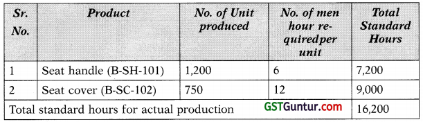
Working Notes 2 – Calculation of monthly budgeted hours
Annual budgeted hour = 1,86,000
Monthly budgeted hour = 1,86,000 hours/12 months = 15,500

Working Notes 3 – Calculation of actual hours for actual production

No.Particulars	Quantum in No.
1. No. of days production function worked	25
2. No. of hour in day	8
3. No. of worker in division	75
Total actual hours for month	15,000

Note – All calculations are on monthly basis.

Question 35.
During September 2020, Sandy offers bundling and item packing facilities (for standard size 24” × 12” × 10”) to give best facility to satisfy its industrial customers ’ need at the Great Ocean Warehouse. Sandy plans to pack 93,750 items at the rate of ₹ 4.50 per item. Sandy estimates that variable cost (all resources) will be equal to ₹ 1.50 per item packed and that fixed costs (rent, electricity, and maintenance charges) will be equal to ₹ 58,000 p.m. In September 2020, Sandy packed 1,12,500 items and received ₹ 5,06,250 as total revenue. However, Sandy paid ₹1,80,000 on resources (including urgent purchase of tape at retail price). In addition, Sandy paid ₹ 70,000 to the warehouse administration for rent, electricity, and maintenance charges. (This past September was unusually hot, and Sandy is charged a percentage of the warehouse’s actual electricity bill.)
Required
PREPARE a budget reconciliation report along with suitable analysis.
Answer:
Workings
The following table show’s Sandy’s budget profit and actual profit for the month of September 2020:

Particulars	Budgeted Profit	Actual Profit
Items packed	93,750	1,12,500
Revenue (₹)	4,21,875	5,06,250
Less: Variable Costs	1,40,625	1,80,000
Contribution Margin (₹)	2,81,250	3,26,250
Less: Fixed Costs	58,000	70,000
Profit (₹)	2,23,250	2,56,250

Analysis
Sandy’s standard selling (packing) price is ₹ 4.50 per item and her standard variable cost is₹ 1.50 per item. Therefore, Sandy’s budgeted revenue = 93,750 × ₹ 4.50 = ₹ 4,21,875 and her budgeted variable costs = 93,750 ×₹ 1.50 =₹ 1,40,625. From the table, we can identify that Sandy’s actual profit for September 2020 was 33,000 higher than his budgeted profit (₹ 2,56,250 – ₹ 2,23,250) ie., Sandy’s total profit variance is ₹ 33,000 (F).

₹Sandy’s sales contribution volume variance equals to the difference between his standard contribution and budgeted contribution. Each item is budgeted to contribute 3.00 toward profit; since Sandy packed 18,750 more items than budgeted, the increase in volume should have contributed ₹ 56,250 = 18,750 × ₹ 3.00 to actual profit. Therefore, Sandy’s sales contribution volume variance is ₹ 56,250 (F).

Sandy’s overall variable cost variance equals to the difference between her standard variable costs and her actual variable costs, or ₹ 1,68,750- ₹ 1,80,000 = ₹ 11.250 (A). But there is not adequate data to segregate Sandy’s variable cost variance into price and quantity elements. To compute these variances, we would require the amount of resources Sandy budgets to use per item packed and the actual & budgeted price of each resource i.e., an adverse variable cost variance can arise as Sandy used more resources per item packed and/or She paid more than budgeted for the resources used). While the issue appears to suggest that Sandy’s adverse variable cost variance arose due to spending more on tape than planned, it is not sure that the entire ₹ 11,250 variance is attributable to this. In fact, it is likely that the tape price variance was greater than ₹ 11,250 (A) and that Sandy had a favourable resource quantity variance to offset this.
Sandy’s fixed cost expenditure variance equals the difference between budgeted and actual fixed costs, or ₹ 58,000 – ₹ 70,000 = ₹ 12,000
We can now prepare the following budget reconciliation report:

Item	Amount (₹)
Budgeted Profit	2,23,250
Sales Volume Variance	56,250 (F)
Variable Cost Variance	11,250 (A)
Fixed Cost Expenditure Variance	12,000 (A)
Actual Profit	2,56,250

Ouestion 36.
Y Ltd., based in Kuala Lumpur, is the Malaysian subsidiary of Japan’s NY corporation, headquartered in Tokyo. Y’s principal Malaysian businesses include marketing, sales, and after-sales service of electronic products & software exports products. Y set up a new factory in Penang to manufacture and sell integrated circuit ‘Q50X-N’. The first quarter’s budgeted production and sales were 2,000 units. The budgeted sales price and standard costs for ‘Q50X-N’ were as follows:

	RM	RM
Standard Sales Price per unit		50
Standard Costs per unit
Circuit X (10 units @ RM 2.5)	25
Circuit Designers (6 hrs. @ RM 2)	12	(37)
Standard Contribution per unit		13

Actual results for the first quarter were as follows:

	RM ’000	RM ’000
Sales (2,000 units)		158
Production Costs (2,000 units)
Circuit X (21,600 units)	97.20
Circuit Designers (11,600 hours)	34.80	(132)
Actual Contribution (2,000 units)		26

The management accountant made the following observations on the actual results-
“In total, the performance agreed with budget; however, in every aspect other than volume, there were huge differences. Sales were made at what was supposed to be the highest feasible price, but we now feel that we could have sold for RM 82.50 with no adverse effect on volume. The Circuit X cost that was anticipated at the time the budget was prepared was RM 2.5per unit. However, the general market price relating to efficient purchases of the Circuit X during the quarter was RM 4.25 per unit. Circuit designers have the responsibility of designing electronic circuits that make up electrical systems. Circuit Designer’s costs rose dramatically with increased demand for the specialist skills required to produce the ‘Q50X-N’, and the general market rate was RM 3.125per hour – although Yalways paid below the normal market rate whenever possible. In my opinion, it is not necessary to measure the first quarter’s performance through variance analysis. Further, our operations are fully efficient as the final contribution is equal to the original budget. ”
Required
COMMENT on management accountant’s view. (10 Marks) [Oct 2020 MTP]
Answer:
Comment
As the management accountant states, and the analysis (W.N.l) presents, the overall variance for the KONI is nil. The cumulative adverse variances exactly offset the favourable variances i.e. sales price variance and circuit designer’s efficiency variance. However, this traditional analysis does not clearly show the efficiency with which the KONI operated during the quarter, as it is difficult to say whether some of the variances arose from the use of incorrect standards, or whether they were due to efficient or inefficient application of those standards.

As seen from W.N. 3, on the cost side, the circuit designer’s rate variance has changed from adverse to favourable, and the price variance for circuit X, while remaining adverse, is significantly reduced in comparison to that calculated under the traditional analysis (W.N.l); on the sales side, sales price variance, which was particularly large and favourable in the traditional analysis (W.N.1), is changed into an adverse variance in the revised approach, reflecting the fact that the KONI failed to sell at prices that were actually available in the market.

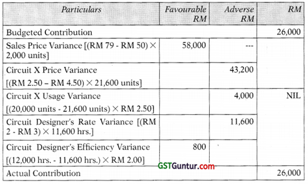
W.N.2
Statement Showing Original Standards, Revised Standards, and Actual Results for Quarter 1

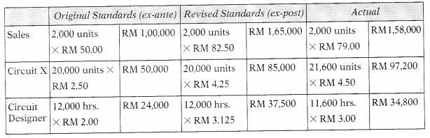
W.N.3

Particulars	(Rs.)	(Rs.)
Operational Variances		16,500 (A)
Sales Price [(RM 79.00 – RM 82.50) × 2,000 units]	7,000 (A)
Circuit X Price [(RM 4.25 – RM 4.50) × 21,600 units]	5,400 (A)
Circuit X Usage [(20,000 units – 21,600 units) × RM 4.25]	6,800 (A)
Circuit Designer Rate [(RM 3.125 – RM 3.00) × 11,600 hrs.]	1,450 (F)
Circuit Designer Efficiency [(12,000 hrs.- 11,600 hrs.) × RM 3.125] ‘	1,250 (F)

W.N.4

Particulars	(Rs.)	(Rs.)
Planning Variance
Sales Price [(RM 82.50 – RM 50.00) × 2,000 units]	65,000 (F)
Circuit X Price [(RM 2.50 – RM 4.25) × 20,000 units]	35,000 (A)	16,500 (F)
Circuit Designer Rate [(RM 2.00 – RM 3.125) × 12,000 hrs.]	13,500 (A)

Question 37.
ZAINA Private Limited is a manufacturing company of electrical equipment. The company is facing the possibility of a strike by its direct production workers engaged on the assembly of one of its machines. The Trade Union is demanding an increase of 8% backdated.
The Machine whose production (Ceiling Fans) would be affected by the strike is sold to distributors at a discount of 25% from the current recommended selling price of ₹ 2,000. The estimated costs for the Ceiling Fans are:

Particulars	Fixed Cost (₹)	Variable Cost (₹)
Production	8,00,000	1,200 Per Ceiling Fan
Distribution	3,00,000	80 Per Ceiling Fan
Total Cost	11,00,000	1,280 Per Ceiling Fan

Direct labour comprises 60% of the variable production cost. The budgeted output is 30,000 Ceiling Fans in 50 working weeks per year. If the strike takes place, the following situations are expected by the company:
(a) Maintenance staff, whose wages are included in the fixed production costs, would used to carry out an overhaul of the conveyor system using materials worth ₹ 50,000. This work would otherwise be undertaken by an outside contractor at a cost including materials ₹ 1,50,000.
(b) Sales of 500 Ceiling Fans would be lost to completion. The balance that could ordinarily have been produced during the strike period, could however, be sold, but these ceiling fans would have to be produced in overtime working which would be at an efficiency rating of 80% of the normal. This would also entail additional fixed costs of ₹ 40,000 and wage payments at time and one-half.
Required
(i) CALCULATE the profit or loss with and without strike.
(ii) Taking, purely economic point of view, ADVISE the management to allow the strike to go ahead, rather than agree to the Union’s demand.
(iii) LIST-Any two factors, not considered in yours above evaluation that may have adverse financial effects for the company, if the strike were to take place. (10 Marks) [Nov. 2020 Exam]
Answer:
(i) Statement Showing the profit or Loss with and without Stirke

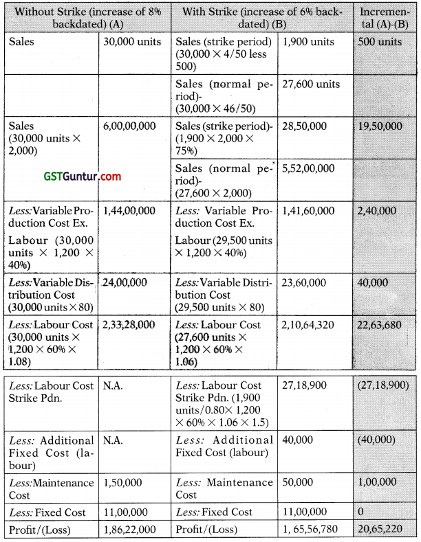
(ii) If there is no strike, it will yield a financial advantage of 20,65,220. Therefore, from a purely economic point of view, management should accept union’s demand.

(iii) These factors, not considered in above evaluation, that may have adverse effects, if the strike were to take place are:

There will be knock on effect of wage increase and all other workers will start demanding it.
Customers gone to competitors may not even return.
Loss of goodwill.
Behavioural effects after strike period and their impact on work.
Strain in relation between trade union, labour, and management.

Question 38.
(Labour Variance & Interpretation)
KRI Sanitation Ltd. manufactures a single product and the standard cost system’ is followed standard cost per unit is calculated as below:

Particulars	Amount (₹ )
Direct Materials (4 kg. @ ₹ 7 kg.)	28
Direct Labour (5 Hours @ ₹ 9 per hour)	45
Variable overheads (6 Hours @ ₹ 2 per hour)	12

The other data for the month of June 2020 is given below:

Particulars	Budgeted	Actual
Production and Sales	15,000 units	₹ 13,800 units
Direct Material	60,000 kg. (a ₹ 7 per kg.	60,000 kg. @ ₹ 7 per kg.
Direct Labour	75,000 Hours @ ₹ 9 per hour	₹ 5,69,600 (for 71,200 hours)
Variable Overheads	1,80,000	1,72,500

Required
(i) CALCULATE following variances:

Direct Labour Rate Variance
Direct Labour Efficiency Variance (3 Marks)

(ii) INTERPRET the result. (7 Marks) [Nov. 2020 Exam]
Answer:
(i) Calculation of Variances →
Labour Rate Variance = Standard Cost of Actual Time – Actual Cost
= (SR × AH) – (AR × AH)
Or
= (SR – AR) × AH
= (₹ 9.00 – ₹ 8.00*) × 71,200 hrs.
= ₹ 71,200(F)
(*) Actual Labour Rate per hour = $\frac{\text { Actual Paid }}{\text { Actual Hours }}$
Actual Paid Actual Hours = $\frac{₹ 5,69,600}{71,200 \mathrm{hrs} .}$
= ₹ 8.00
Labour Efficiency Variance = Standard Cost of Standard Time for Actual Production – Standard Cost of Actual Time
= (SH × SR) – (AH × SR)
Or
= (SH – AH) × SR
= (69,000$ hrs. – 71,200 hrs.) × ₹ 9.00
= ₹ 19,800 (A)
($) Standard Hours = Actual Production × Std. hrs. per unit
= 13,800 units × 5 hrs.
= 69,000 hrs.

(ii) Interpretation of Variances →
The favourable rate variance indicates that expenditure was 71,200 less than the standard because a lower than standard rate was paid for each hour of labour (i.e. ₹ 8 per hr. against ₹ 9 per hr.), this could mean that I less skilled labour was used than provided for in the standard; and this then lowered efficiency with the result that the efficiency was lower than expected, result in adverse efficiency variance of ₹ 19,800; and perhaps poor materials handling and high rates of rejections too (this is indicated by adverse material usage variance of ₹ 33,600. This throughout analysis shows a positive impact of ₹ 17,800 on profit for which labour rate variance is the main contributor.
Workings
Material Usage Variance = Standard Cost of Standard Quantity for Actual Production – Standard Cost of Actual Quantity
= (SQ × SP) – (AQ × SP)
Or
= (SQ – AQ) × SP
= (52,000$ kg. – 60,000 kg) × ₹ 7.00
= ₹ 33,600
Standard Quantity = Actual Production × Std. Qty. per unit
= 13,800 units × 4 kg.
= 55,200 kg.
Not-Ignored Variables Overheads.

Alternative
Interpretation of Variances
The favourable rate variance indicates that expenditure was 71,200 less than the standard because a lower than standard rate was paid for each hour of labour (i.e. ₹ 8 per hr. against ₹ 9 per hr.), this could mean that
(i) Less skilled labour was used than provided for in the standard.
(ii) Fall in the overall wage rates in the market due to an increase in the supply of labour.
(iii) Inappropriately high setting of the standard cost of direct labour which may be attributed to inaccurate planning.
Labour efficiency variance of 19,800(A) means that efficiency was lower than expected or more actual labour hours required than standard labour hours. The reasons may include:
(i) Hiring of lesser skilled labour than the standard.
(ii) Achieving Lower learning curve during the period than anticipated in the standard.
(iii) Idle time incurred during a period caused by disruption or stoppage of work. Poor materials handling and high rates of rejections also affects labour efficiency.
In a nutshell, due to Lower labour rate variance (Fav), labour efficiency (Adv) has come down.

Question 39.
(Reconciliation between Budgeted Profit and Actual Profit)
Sri Manufacturers Ltd. manufactures a single product. Standard cost per unit is as follows:

Particulars		₹
Materials	12 kgs × ₹ 5 per kg	60
Labour	10 hrs × ₹ 7per hour	70
Variable Overheads	10 hrs × per hour	30
Fixed Overheads	10 hrs × per hour	30
Profit		60
Selling Price		250

Overheads are allocated on the basis of direct labour hours. In the month of March 2020 there was no difference between the budgeted and actual selling price and there was no opening and closing stock during the period.
The other details for the month of March 2020 are as under:

	Budgeted	Actual
Product and sales	2,500 units	2,000 units
Direct Materials	30,000 kgs @ 5 per kg	30,000 kgs @ 5 per kg
Direct Labour	25,000 hrs @ ₹ 7 per hour	22,500 hrs @ ₹ 7 per hour
Variable Overheads	₹ 75,000	₹ 67,500
Fixed Overheads	₹ 75,000	₹ 75,000

Required
RECONCILE the budgeted and actual profit with the help of variances according to each of the following methods:
(i) The conventional method (3 Marks)
(ii) The relevant cost method assuming that
(a) Materials are scarce and are restricted to supply of 30,000 kgs for the period. (3 Marks)
(b) Labour hours are limited and available hours are only 25,000 hours for the period. (4 Marks) [Jan 2021 Exam]
Answer:
Computation of Variances
Material Usage Variance
= Standard Price × (Standard Quantity – Actual Quantity)
= ₹ 5.00 × (24,000 Kgs. – 30,000 Kgs.)
= ₹ 30,000 (A)

Labour Efficiency Variance
= Standard Rate × (Standard Hours – Actual Hours)
= ₹ 7.00 × (20,000* hrs. – 22,500 hrs.)
= ₹ 17,500 (A)

Fixed Overhead Volume Variance
Absorbed Fixed Overheads – Budgeted Fixed Overheads
= (20,000 hrs. × ₹ 3.00) – (25,000 hrs. × ₹ 3.00)
= ₹ 15,000 (A)

Sales Margin Volume Variance = Standard Margin – Budgeted Margin
= (2,000 units × ₹ 60.00) – (2,500 units × ₹ 60.00)
= ₹ 30,000 (A)

Sales Contribution Volume Variance
= Standard Contribution – Budgeted Contribution
= (2,000 units × ₹ 90.00) – (2,500 units × ₹ 190.00)
= ₹ 45,000 (A)

Statement Showing “Reconciliation between Budgeted
Profit & Actual Profit”

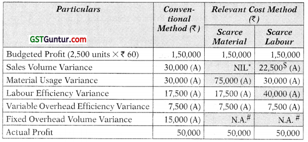
Notes
Scarce Material
Based on conventional method, direct material usage variance is ₹ 30,000 (A) i.e., 6,000 Kg. × ₹ 5. In this situation material is scarce, and, therefore, material cost variance based on relevant cost method should also include contribution lost per unit of material. Excess usage of 6,000 Kg. leads to lost contribution of ₹ 45,000 i.e., 6,000 Kgs. × ₹ 7.5. Total material usage variance based on relevant cost method, when material is scarce will be: ₹ 30,000 (A) + ₹ 45,000 (A) = ₹ 75,000 (A). Since labour is not scarce, labour variances are identical to conventional method.

Excess usage of 6,000 Kgs. leads to loss of contribution from 500 units i.e., ₹ 45,000 (500 units × ₹ 90). It is not the function of the sales manager to use material efficiently. Hence, loss of contribution from 500 units should be excluded while computing sales contribution volume variance.
(*)→ Therefore, sales contribution volume variance, when materials are scarce will be NIL i.e., ₹ 45,000 (A) – ₹ 45,000 (A).

Scarce Labour
Material is no longer scarce, and, therefore, the direct material variances are same as in conventional method. In conventional method, excess labour hours used are: 20,000 hrs. – 22,500 hrs. = 2,500 hrs. Contribution lost per hour = 1 9. Therefore, total contribution lost, when labour is scarce will be:
2,500 hrs. × ₹ 19 = ₹ 22,500. Therefore, total labour efficiency variance, when labour hours are scarce will be 140,000 (A) i.e., ₹ 17,500 (A) + ₹ 22,500 (A).

Excess usage of 2,500 hrs. leads to loss of contribution from 250 units i.e., ₹ 22,500 (250 units × ₹ 90). It is not the function of the sales manager to use labour hours efficiently. Hence, loss of contribution from 250 units should be excluded while computing sales contribution volume Variance,
($)→ Therefore, sales contribution volume variance, when labour hours are scarce will be 122,500 (A) i.e., ₹ 45,000 (A) – ₹ 22,50Q (A).
Fixed Overhead Volume Variance:
(#) → The fixed overhead volume variance does not arise in marginal costing system. In absorption costing system, it represents the value of the under or over absorbed fixed overheads due to change in production volume. When costing is in use there is no overhead volume variance, because 4 marginal costing does not absorb fixed overheads.

Question 40.
(Reconciliation}
Williams Footwear (WF)is a shop that focuses on shoes for various sports I and activities like jogging, cricket, tennis, oral hockey. Budgeted profit for the WF is calculated considering an average selling price of ₹ 500 per pah of shoes and an average cost of ₹ 350 per pair of shoes. The super visor of the WF has discretion in staffing and in setting prices. Usually, the WF is staffed for 65G hrs per month ai a badgered rate of ₹ 125 per hr. In addition to this base wages, sales staff gas a payment equal to 5.Sts of takings, Moreover, staffing levels are not expected, to change in response to “little’ changes in shoe sales. For Sep’ 2021, the IFF had budgeted sales of 2,250 pairs of shoes and 650 staffing hrs.
Actual results for Sep’2021 were as follows:

Pairs of shoes sold	2,500
Revenue	12,00,000
Less: Cost of shoes	8,25,000
Less: Staff – additional payment	66,000
Less: Staff – base wages @ 1 125 per hour	78,125
Profit	₹ 2,30,875
Note – little” changes in shoe sales specified as ± 12%.

Required
(i) PREPARE a reconciliation statement of budgeted profit to actual profit.
(ii) COMMENT on supervisor’s performance. [Nov 2021 RTP]
Answer:
(i) Reconciliation Statement Budgeted and Actual Profit (Sep’ 2021)

Budgeted profit	1,94,375
Sales volume variance (F)	30,625
Sales price variance (A)	50,000
Shoe cost variance (F)	50,000
Staff cost variance-commission (F)	2,750
Staff cost variance-base wage (F)	3,125
Actual profit	₹ 2,30,875

The performance seems good. It shows that the supervisor of the WF passed on a 5.7% decrease in shoe cost to customers (same is also revealed through the entirely offsetting of the shoe cost variance and price variance), ie. shoe costs decreased by ₹20 per pair, from a standard cost of ₹ 350 per pair to an actual cost ₹330 per pair. Additionally, the selling price decreased by ₹20 per pair, from a standard price of ₹ 500 per pair to an actual price of ₹480 per pair. In turn, the reduction in the selling price appeared to produce a favourable sales volume variance and a reasonable increase in profit.
Since the reduction in the selling price, staff commissions also were lower than budgeted. Moreover, the ₹50,000 reduction in revenue led to 0.055 × ₹ 50,000 = ₹2,750 less in commission costs.
Lastly, staffing was 25 hours under budget, leading to a savings of 25 × ₹ 125 = ₹3,125. Therefore, the supervisor attained an increase in sales with lesser staff hours.
Overall, it appears that the manager has done a great job of making revenue and controlling costs.
Workings
Statement Showing Budgeted and Actual Profit (Sep’ 2021)

	Budgeted Data	Actual Data
Units (pairs of shoes)	2,250	2,500
Price per pair of shoes	₹ 500.00	₹ 480.00
Cost per pair of shoes	₹ 350.00	₹ 330.00
Commission rate	₹ 27.50 (5.5% of ₹ 500)	₹ 26.40 (5.5% ₹480)
Contribution	₹ 122.50	₹ 123.60
Revenue	₹ 11,25,000	₹ 12,00,000
Less: Cost of shoes	7,87,500	8,25,000
Less: Staff – additional payment (commission)	61,875	66,000
Less: Staff – base wages	81,250	78,125
Profit	₹ 1,94,375	₹ 2,30,875

Computation of variances
Total Profit Variance = ₹ 2,30,875 – ₹ 1,94,375
= ₹ 36,500 (F)

Sales Contribution Volume Variance = StandardContribution-Budgeted Contribution
= ₹ 122.50 × ₹ 2,500 – ₹ 122.50 ₹ 2,250
= ₹ 3,06,250 – ₹ 2,75,625 = ₹ 30,625 (F)

Sales Price Variance = Actual Revenue – Standard Revenue
= ₹ 480 × 2,500 – ₹ 500 × 2,500
= ₹ 12,00,000 – ₹ 12,50,000 = ₹ 50,000 (A)

Shoe Cost Variance*
= ₹ 350 × 2,500 – ₹330 × 2,500
= ₹ 8,75,000 – ₹ 8,25,000 = ₹ 50,000 (F)

Staff Cost Variance-commission*
= ₹ 27.50 × 2,500 – ₹ 26.40 × 2,500
= ₹ 68,750 – ₹ 66,000 = ₹2,750

Staff Cost Variance (base wage) = ₹81,250 – ₹78,125 = ₹3,125(F).
(*) Note- The cost variance (for both shoe and staff-commission) equal to the difference between the standard cost and the actual cost.

Standard Costing – CA Final SCMPE Study Material

Leave a Comment Cancel Reply