Dividend Decisions – CA Inter FM Notes

Dividend Decisions– CA Inter FM Notes is designed strictly as per the latest syllabus and exam pattern.

Dividend Decisions– CA Inter FM Notes

1. Theories of Dividend:

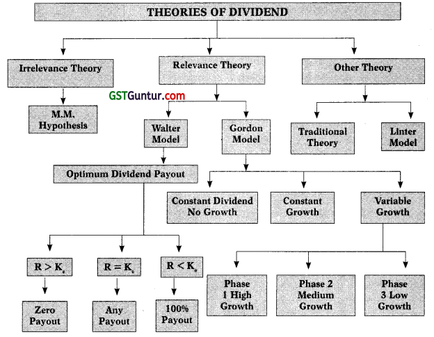
2. Modigliani and Miller (MM) Hypothesis (1961): MM approach is in support of the irrelevance of dividends Le. firm’s dividend policy has no effect on either the price of a firm’s stock or its cost of capital.

Assumptions:

• Perfect capital markets
• No taxes or no tax discrimination
• Fixed investment policy
• No floatation or transaction cost
• Risk of uncertainty does not exist

Steps in Practical Problems:
Step 1: Calculate P₁:
P₀ = \(\frac{\mathrm{P}_1+\mathrm{D}_1}{1+\mathrm{K}_{\mathrm{e}}}\) or P₀
Step 2: Calculate New Shares (∆n) required to be issued:
∆n = \(\frac{\text { Funds Required }}{\mathrm{P}_1}\) = \(\frac{\mathrm{I}-(\mathrm{E}-\mathrm{D})}{\mathrm{P}_1}\)
Step 3: Calculate Value of Firm (nP0):
nP₀ = \(\frac{(\mathrm{n}+\Delta \mathrm{n}) \mathrm{P}_1-\mathrm{I}+\mathrm{E}}{1-\mathrm{K}_{\mathrm{c}}}\)

3. Walter Model: Walter approach is in support of the relevance of dividends le. firm’s dividend policy has effect on either the price of a firm’s stock or its cost of capital.

Assumptions:

• All investment proposals of the firm are to be financed through retained earnings only
• ‘r’ rate of return & ‘K_e‘ cost of capital are constant
• Perfect capital markets
• No taxes or no tax discrimination between dividend income and capital appreciation (capital gain)
• No floatation or transaction cost
• The firm has perpetual life

Formula:
Market Price of Share (P) = \(\frac{\mathrm{D}+\frac{\mathrm{r}}{\mathrm{K}_{\mathrm{e}}}(\mathrm{E}-\mathrm{D})}{\mathrm{K}_{\mathrm{e}}}\)
Where,
P = Market Price of the share
E = Earnings per share
D = Dividend per share
K_e = Cost of equity/rate of capitalization/discount rate
R = Internal rate of return/return on investment

Company	‘r’ VS ‘Ke‘	Optimum Dividend Payout
Growth	r > Ke	Zero
Constant	r = Ke	Every payout ratio is optimum
Decline	r < Ke	100%

4. Gordon ‘s Model: According to Gordon’s model dividend is relevant and dividend policy of a company affects its value.

Assumptions:

• Firm is an all equity firm.
• IRR will remain constant.
• K_e will remains constant.
• Retention ratio (b) is constant i.e. constant dividend payout ratio will be followed
• Growth rate (g = br) is also constant.
• K_e > g
• All investment proposals of the firm are to be financed through retained earnings only.

Formulae of MPS {Gordon’s Model or Dividend Discount Model (DDM)}:
Situation 1: Zero Growth or Constant Dividend:
P₀ = \(\frac{\mathrm{D}}{\mathrm{K}_{\mathrm{e}}}\)

Situation 2: Constant Growth:
P₀ = \(\frac{D_1}{\mathrm{~K}_{\mathrm{e}}-\mathrm{g}}\) or = \(\frac{\mathrm{D}_0(1+\mathrm{g})}{\mathrm{K}_{\mathrm{e}}-\mathrm{g}}\)
g = b (earning retention ratio) × r (IRR or ROE)

Situation 3: Variable Growth:

• Phase 1: Very High Growth
• Phase 2: High Growth
• Phase 3: Average Growth equal to industry

P₀ = Present Value of all future benefit from share
Note: Calculation of Intrinsic value of share and MPS of share are same

Company	‘r’ VS ‘Ke‘	Optimum Dividend Payout
Growth	r > Ke	Zero
Constant	r = Ke	Every payout ratio is optimum
Decline	r < Ke	100%

5. The ‘Bird-in-hand theory’: Myron Gordon revised his dividend model and considered the risk and uncertainty in his model. The Bird-in-hand theory of Gordon has two arguments:

• Investors are risk averse and
• Investors put a premium on certain return and discount on uncertain return.

Investors are rational, they want to avoid risk and uncertainty. They would prefer to pay a higher price for shares on which current dividends are paid. Conversely, they would discount the value of shares of a firm which postpones dividends. The discount rate would vary with the retention rate.

6. Traditional Model: According to the traditional position expounded by Graham & Dodd, the stock market places considerably more weight on divi-dends than on retained earnings. Their view is expressed quantitatively in the following valuation model:
P = m \(\left(D+\frac{E}{3}\right)\)
Where,
P = Market price per share
D = Dividend per share
E = Earnings per share
M = a multiplier

7. John Linter’s Model: Linter’s model has two parameters:

• The target payout ratio,
• The spread at which current dividends adjust to the target.

D₁ = D₀ + [(EPS × Target payout) – D₀] × Af
Where,
D₁ = Dividend in year 1
D₀ = Dividend in year 0 (last year dividend)
EPS = Earnings per share
Af = Adjustment factor or Speed of adjustment

8. Stock Splits: Stock split means splitting one share into many. Stock splits is a tool used by the companies to regulate the prices of shares i.e. if a share price increases beyond a limit, it may become less tradable, for e.g. suppose a company’s share price increases from ₹ 50 to ₹ 1000 over the years, it is possible that it might goes out of range of many investors.

Advantages:

• It makes the share affordable to small investors.
• Number of shares may increase the number of shareholders, hence the potential of investment may increase.

Limitations:

• Additional expenditure need to be incurred on the process of stock split.
• Low share price may attract speculators or short-term investors, which are generally not preferred by any company.