Price Determination in Different Markets – CA Foundation Economics Notes Chapter 4

Browsing through CA Foundation Business Economics Notes Chapter 4 Price Determination in Different Markets help students to revise the complete subject quickly.

Price Determination in Different Markets – Business Economics CA Foundation Notes Chapter 4

Meaning of market:
→ In ordinary language, a market refers to a place where the buyers and sellers of a commodity gather and strike bargains.

→ In economics, however, the term “Market” refers to a market for a commodity.
Example – Cloth market; furniture market; etc.

→ According to Chapman, “the term market refers not necessarily to a place and always to a commodity and buyers and sellers who are in direct competition with one another”.

→ According to the French economist Cournot, “Market is not any particular place in which things are bought and sold, but the whole of any region in which buyers and sellers are in such free intercourse with each other that the prices of the same goods tend to equality easily and quickly”.

→ The above mentioned definitions reveals the following features of a market:

• A region. A market does not refer to a fixed place. It covers a region, which may be a town, state, country or even world.
• Existence of buyers and sellers. Market refers to the network of potential buyers and sellers who may be at different places.
• Existence of commodity or service. The exchange transactions between the buyers and sellers can take place only when there is a commodity or service to buy and sell.
• Bargaining for a price between potential buyers and sellers.
• Knowledge about market conditions. Buyers and sellers are aware of the prices offered or accepted by other buyers and sellers through any means of communication.
• One price for a commodity or service at a given time.

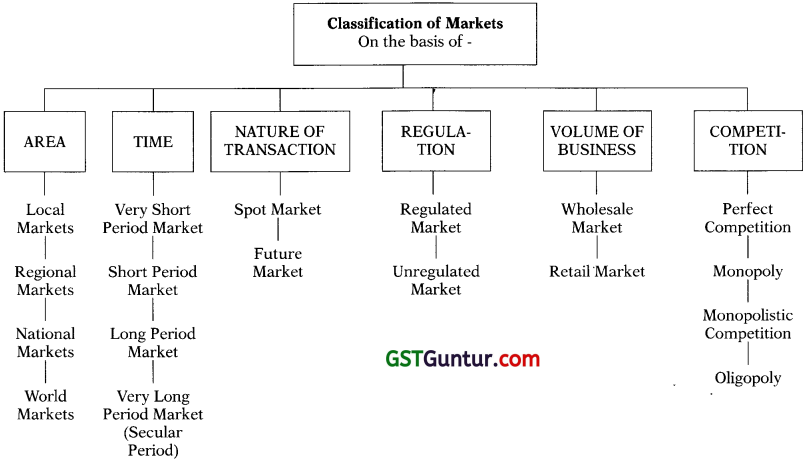
Classification of Market:
Markets may be classified on the basis of different criteria. In Economics, generally the classification is made as pointed out in the following chart –

Price Determination in Different Markets:

Types of market structures:
→ Market can be classified on the basis of area, volume of business, time, status of sellers, regulation and control.

→ The main types of markets can be summed up as follows :
1. Perfect Competition :

• Perfect competition market is one where there are many sellers selling identical products to many buyers at a uniform.

2. Monopoly:

• Monopoly market structure is a market situation in which there is a single seller of a commodity selling to many buyers.
• The commodity has no close substitutes available.
• A monopolist therefore, has a considerable influence on the price and supply of his commodity.

3. Monopolistic Competition :
Monopolistic competition is a market situation in which there are many sellers selling differentiated goods to many buyers.

4. Oligopoly:
Oligopoly is a market situation in which there are few sellers selling either homogeneous or differentiated goods.

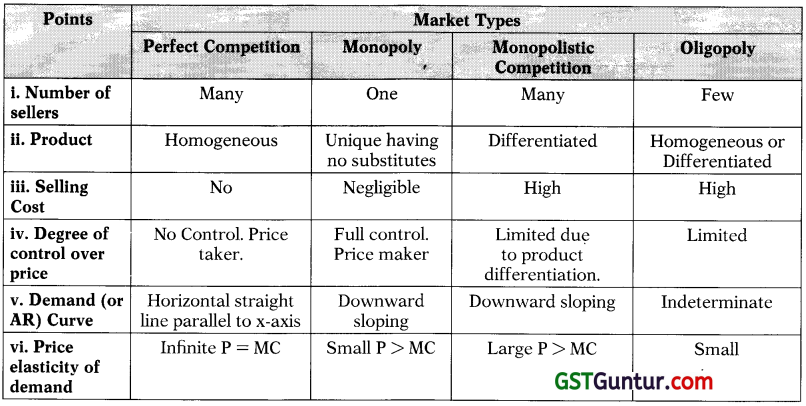
Table : Features of major types of markets

Concepts of total revenue, average revenue and marginal revenue:
Total Revenue : (TR)

• Total revenue may be defined as the total amount of money received by the firm by selling a certain units of a commodity.
• It is obtained by multiplying the price per unit of a commodity with the total number of units sold.
• Total Revenue = Price per unit X Total No. of units sold
  TR = P X Q
• Example – A firm sells 100 units of a commodity @ ₹ 15 each, then its total revenue is ₹ 15 X 100 units = ₹ 1,500

Average Revenue : (AR)
→ Average revenue is the revenue per unit of the commodity sold.

→ It is simply the total revenue divided by the number of units of output sold.

→ Average Revenue = \(\frac { Total Revenue }{ No.of units sold }\)
AR = \(\frac { TR }{ Q }\)

→ Example – A firm earns total revenue of ₹ 2,000 by the sale of 100 units of a commodity, then its average revenue is ₹ 20 (₹ 2000 ÷ 100 units)

→ By definition average revenue is the price per unit of output. To prove it –
∴ AR = \(\frac { TR }{ Q }\), since TR = P x Q
AR = \(\frac { P×Q }{ Q }\)
∴ AR = P (Price)

Marginal Revenue (MR):
→ Marginal revenue refers to the addition to total revenue by selling one more unit of a commodity.

→ Marginal revenue may also be defined as the change in total revenue resulting from the sale of one more unit of a commodity

→ Example – If a firm sells 100 units of a commodity @ ₹ 15 each, its TR is ₹ 1,500. Now, if it increases the sale by ten units i.e. it sells 110 units @ ₹ 14 each, its TR is ₹ 1,540. Thus,
MR = \(\frac { ∆ TR }{ ∆ Q }\)

→ Where – ∆ TR is the change in total revenue
∆ Q is the change in the quantity sold

→ For one unit change – MRn = TRn – TRn-₁
Where
MRn = Marginal Revenue from ‘n’ units
TRn = Total Revenue of ‘n’ units
TRn-₁ = Total Revenue from ‘n-1’ units
n = any give number

Marginal revenue, average revenue, total revenue and elasticity of demand:
→ The relationship between AR, MR and price elasticity of demand can be examined with the formula –
MR = AR x \(\frac { e – 1 }{ e }\)
Where, e = price elasticity of demand.
If e = 1, MR = 0
If e > 1, MR will be positive i.e. MR > 0
If e < 1, MR will be negative i.e. MR < 0

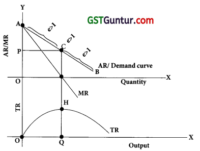
The relationship between AR, MR, TR & elasticity of demand.

→ The above figure reveals the following on a straight line demand curve (or AR curve):

• When e > 1, marginal revenue is positive and therefore total revenue is rising,
• When e = 1, marginal revenue is zero and therefore total revenue is maximum, and
• When e < 1, marginal revenue is negative and therefore total revenue is falling.

Behavioural Principles:

• Principle 1 : A firm should not produce at all if its total revenue is either equal to or less than its I total variable cost.
• Principle 2 : It will be profitable for the firm to expand output so long as marginal revenue is more than marginal cost till the point where marginal revenue equals marginal cost.

Also the marginal cost curve should cut its marginal revenue curve from below.

Determination of prices:

Determination of equilibrium price:
→ We know that law of demand reveals, if other conditions remain unchanged, more quantity | of a commodity is demanded in the market at a lower price and less quantity is demanded at a higher price. Therefore, demand curve slopes downward.

→ Similarly, the law of supply reveals, if other conditions remain unchanged, more quantity of a commodity is supplied in the market at a higher price and less quantity is supplied at a lower price. Therefore, supply curve slopes upward.

→ Demand and supply are the two main factors that determine the price of a commodity in the market. In other words, the price of a commodity is determined by the inter-action of the forces of demand and supply.

→ The price that will come to prevail in the market is one at which quantity demanded equals 1 quantity supplied.

→ This price at which quantity demand equals quantity supplied is called equilibrium price.

→ The quantity demanded and supplied at equilibrium price is called equilibrium quantity.

→ The process of price determination is illustrated with the help of following imaginary schedule and diagram.

Table – Determination of Price:
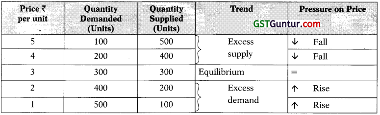The The above table shows that at a price of ₹ 3 per unit, the quantity demanded equals quantity supplied of the commodity. At ₹ 3 two forces of demand and supply are balanced. Thus, ₹ 3 is the equilibrium price and equilibrium quantity at ₹ 3 is 300 units.

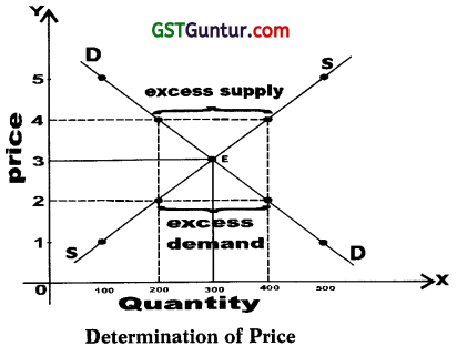
→ The equilibrium between demand and supply can also be explained graphically as in Fig.

→ In Fig – the market is at equilibrium at point ‘E’, where the demand curve and supply curve intersect each other. Here quantity demanded and supplied, are equal to each other.

→ At point ‘E’, the equilibrium price is ₹ 3 per unit and equilibrium quantity is 300 units.

→ If the price rises to ₹ 4 per unit, the supply rises to 400 units but demand falls to 200 units. Thus, there is excess supply of 200 units in the market.

→ In order to sell off excess supply of 200 units the sellers will compete among themselves and in doing so the price will fall.

→ As a result the quantity demand will rise and quantity supplied will fall and becoming equal to each other at the equilibrium price ₹ 3.

→ Similarly, if the price falls to ₹ 2 per unit, the demand rises to 400 units but supply falls to 200 units. Thus, there is excess demand of 200 units in the market.

→ As the price is less there is competition among the buyers to buy more and more. This competition among buyers increases with the entry of new buyers.

→ More demand and less supply and competition among buyers will push up the price.

→ As a result, quantity demanded will fall and quantity supplied will rise and become equal to each other at the equilibrium price of ₹ 3.

Effects of shifts in demand and supply on equilibrium price:
→ While determining the equilibrium price, it was assumed that demand and supply conditions were constant. In reality however, the condition of demand and supply change continuously.

→ Thus, changes in income, taste and preferences, changes in the availability and prices of related goods, etc. brings changes in demand conditions and cause demand curve to shift either to right or left.

→ In the same way, changes in the technology, changes price of labour, raw materials, etc., changes in the number of firms, etc. brings changes in supply conditions and cause supply curve to shift either to right or left.
(a) Change (shift) in Demand and Supply remaining constant:

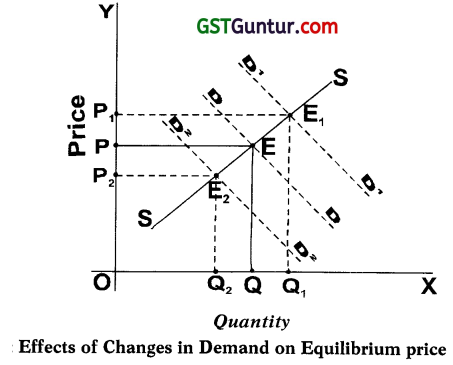
→ In Fig.- DD and SS are the original demand and supply curves respectively inter-secting each other at point E.

→ At point E, the equilibrium price is OP and the demand and supply (ie. equilibrium quantity) are equal at OQ.

→ When the demand increases, the demand curve shifts upwards from DD to D₁D₁, supply remaining the same.

→ As a result, the equilibrium price rises from OP to OP₁, and the equilibrium quantity increases from OQ to OQ₁ as shown at point E₁.

→ When the demand decreases, the demand curve shifts downwards from DD to D₂ D₂, Supply remaining the same.

→ As a result, the equilibrium price falls from OP to OP₂ and the equilibrium quantity decreases from OQ to OQ₂ as shown at point E₂

(b) Change (shift) in Supply and Demand remaining constant:

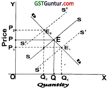
Effects of Changes in Supply on Equilibrium Price.
→ In Fig. – DD and SS are the original demand and supply curves respectively inter-sections each other at point E.

→ At point E, the equilibrium price is OP and the demand and supply (i.e. Equilibrium quantity) are equal at OQ.

→ When the supply increases, the supply curve shifts to the right from SS to S₁ S₁, demand remaining the same.

→ As a result, the equilibrium price falls from OP to OP₁, and the equilibrium quantity increases from OQ to OQ₁, as shown at point E₁.

→ When the supply decreases, the supply curve shifts to the left from SS to S₂ S₂, demand remaining the same.

→ As a result, the equilibrium price rises from OP to OP₂ and the equilibrium quantity decreases from OQ to OQ₂ as shown at point E₂.

Effects of simultaneous shifts in demand and supply on equilibrium price:
Sometimes demand and supply conditions may change at the same time changing the equilibrium price and quantity. The changes in both demand and supply simultaneously can be discussed with the help of following diagrams :

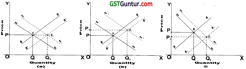
Effect of simultaneous changes in Demand & Supply on Equilibrium Price.
→ In Fig. – DD and SS are the original demand and supply respectively intersecting each other at point E at which the equilibrium price is OP and the equilibrium quantity is OQ.

→ Fig. (a) shows that the increase in demand is equal to increase in supply. The new curves D₁, D₁, and S₁, S₁, intersect at E₁. Therefore, the new equilibrium price is equal to old equilibrium price OP. But equilibrium quantity increases.

→ Fig. (b) shows that the increase in demand is more than increase in supply. The new curves D₁, D₁, and S₁, S₁, intersect each other at point E₁, which shows that new equilibrium price OP₁, is higher than old equilibrium price OP. But equilibrium quantity increases.

→ Fig. (c) shows that the increase in supply is more than increase in demand. The new curves D₁D₁, and S₁S₁ intersect each other at point E₁ which shows that new equilibrium price OP₁ is lower than old equilibrium price OP. But equilibrium quantity increases.

Perfect competition:
Introduction :
→ Perfect competition is a market structure where there are large number of firms (seller) which produce and sell homogeneous product. Individual firm produces only a small portion of the total market supply.

→ Therefore, a single firm cannot affect the price.

• Price is fixed by industry.
• Firm is only a price taker.
• So the price of the commodity is uniform.

Features of perfect competition.
→ Following are the main features of perfect competition :
(1) Large number of buyers and sellers :

• The number of buyers and sellers is so large that none of them can influence the price in the market individually.
• Price of the commodity is determined by the forces of market demand and market supply.

(2) Homogeneous Product:
The product produced by all the firms in the industry are homogeneous.

• They are identical in every respect like colour, size, etc.
• Products are perfect substitutes of each other.

(3) Free entry and exit of the firms from the markets :

• New firms are free to enter the industry any time.
• Old firms or loss incurring firms can leave industry any time.
• The condition of free entry and exit applies only to the long run equilibrium of the industry.

(4) Perfect knowledge of the market:

• Under perfect competition, all firms (sellers) and buyers have perfect knowledge about the market.
• Both have perfect information about prices at which commodities can be sold and bought.

(5) Perfect mobility :
The factors of production can move freely from one occupation to another and from one place to another.

(6) No transport cost:
Transport cost is ignored as all the firms have equal access to the market.

(7) No selling cost:

• Under perfect competition commodities traded are homogeneous and have uniform price.
• Therefore, firm need not make any expenditure on publicity and advertisement.

Equilibrium of the Industry :
→ Industry is a group of firms producing identical commodities.

→ Under perfect competition, price of a commodity is determined by the interaction between market demand and market supply of the whole industry.

→ The equilibrium price is determined at a point where demand for and supply of the whole industry are equal to each other.

→ No individual firm can influence the price.

→ Firm has to accept the price determined by the industry.

→ Therefore, the firm is said to be price taker and industry, the price maker.

→ Equilibrium of the industry is illustrated as follows :
Table – Price Determination:

Industry
Price ₹ Per unit	Demand (Units)	Supply (units)
10 8642	20 40 60 80 100	100 80 60 40 20

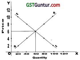
Figure : Equilibrium Price (Industry)
→ The above table and fig. shows that at a price of ₹ 6 per unit, the quantity demanded equals quantity supplied.

→ The industry is at equilibrium at point ‘E’, where the equilibrium price is ₹ 6 and equilibrium quantity is 60 units.

Equilibrium of a firm:
→ We have already seen that under the perfect competition, the price of the commodity is determined by the forces of market demand and market supply i.e. price is determined by industry.

→ Individual firm has to accept the price determined by the industry. Hence, firm is a Price taker.
Table – Equilibrium price (Industry)
→ In the table – the equilibrium price for the industry has been fixed at ₹ 6 per unit through the inter-action of market demand and supply.

→ Table – shows that the firm has no choice but to accept and sell their commodity at a price that has been determined by the industry i.e. ₹ 6 per unit.

→ The firm cannot charge higher price than the market price of ₹ 6 per unit because of fear of loosing customers to rival firms.

→ There is no incentive for the firm to lower the price also.

→ Firm will try to sell as much as it can at the price of ₹ 6 per unit.

→ Table – shows that firm’s AR = MR = Price.

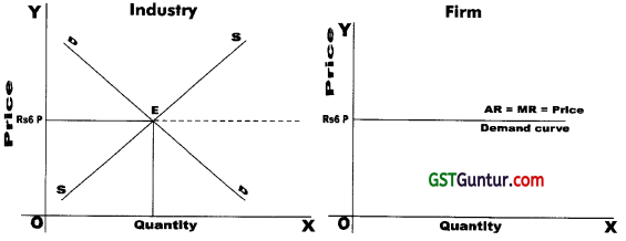
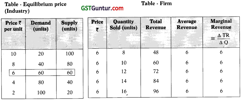
Figure : The firm’s demand curve, AR and MR curves under perfect competition.

→ Fig. shows that being a price taker firm, it has to sell at a given price i.e. 16 per unit.

→ Therefore, firm’s demand curve is a horizontal straight line parallel to X-axis i.e. a perfectly elastic demand curve.

→ We know that price of a commodity is also the AR for the firm.

→ Therefore, demand curve also shows the AR for different quantities sold by the firm.

→ As every additional unit is sold at a given price i.e. ₹ 6 per unit, the MR = AR and the two curves coincides.

→ Thus, in a perfectly competitive market a firm’s
AR = MR = Price = Demand Curve

Conditions for equilibrium of a firm :
→ In perfect competition, the firms are price takers and output adjusters.

→ This is because the price of the commodity is determined by the forces of market demand and market supply i.e. by whole industry and individual firm has to accept it.

→ Therefore firm has to simply choose that level of output which yields maximum profit at the prevailing prices.

→ The firm is at equilibrium when it maximises its profit.

→ The output which helps the firm to maximise its profit is called equilibrium output.

→ There are two conditions for the equilibrium of a firm.
They are –

• Marginal Revenue should be equal to the marginal cost i.e. MR = MC. (First order condition)
• Firm’s marginal cost curve should cut its marginal revenue curve from below i.e. marginal cost curve should have positive slope at the point of equilibrium. (Second order condition)

→ If MR > MC, there is incentive to produce more and add to profits.

→ If MR < MC, the firm will have to decrease the output as cost of production of additional units is high.

→ When MR = MC, it is equilibrium output which maximises the profits.

→ Fig. shows that OP is the price determined the industry and firm has to accept it.

→ At prevailing price OP the firm faces horizontal demand curve or average revenue curve.

→ Since the firm sells every additional unit at the same price, marginal revenue curve coincides with average revenue curve.

→ In the fig. at point ‘A’,
MR = MC
but second condition is not fulfilled.

→ Therefore, OQ₁ is not equilibrium output. Firm should expand output beyond OQ₁ because

• it will result in the fall of marginal cost, and
• add to firm’s profits.

→ In the fig. at point ‘B’ not only
MR = MC
but MC curve cuts the MR curve from below Le. it has positive slope.

→ Therefore, OQ₂ is the equilibrium level of output and point ‘B’ represents equilibrium of firm.

Supply curve of the firm in a competitive market:
In a perfectly competitive industry, the MC curve of the firm is also its supply curve. This can be explained with the help of following figure.

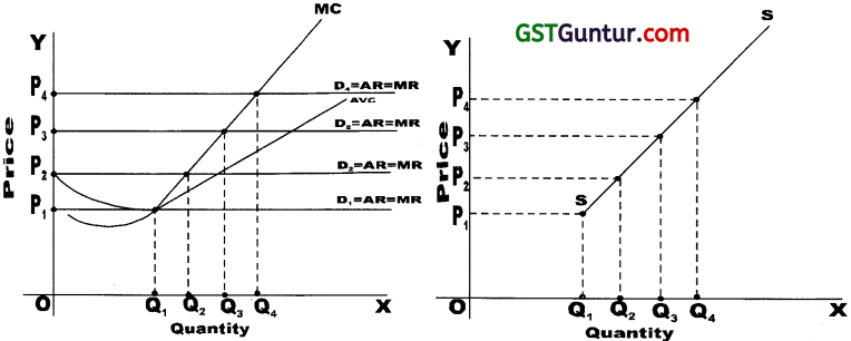
Figure : Marginal Cost and Supply curve of a competitive firm

• The fig. shows that at the market price OP₁, the firm faces demand curve D₁.
• At OP₁, price the firm supplies OQ₁, quantity because here MC = MR.
• If the price rises to OP₂ the firm faces demand curve D₂.
• At OP₂ price the firm supplies OQ₂ quantity.
• Similarly at OP₃ and OP₄ price corresponding supplies are OQ₃ and OQ₄ respectively.
• Thus, the firm’s marginal cost curve indicates the quantities of output which it will supply at different prices.
• It can be observed that the competitive firm’s short run supply curve is identical only with that portion of
• MC curve, which lies above the AVC.
• Hence, price ≥ AVC.

Short Run Equilibrium of a Competitive Firm. (Price – Output Equilibrium):
→ A competitive firm in the short run attains equilibrium at a level of output which satisfies the following two conditions:

• MC = MR, and
• MC curve cuts the MR curve from below.

→ When a competitive firm, is in short run equilibrium, it may find itself in any of the following situations –

• it break evens i.e. earn NORMAL PROFITS where Average Revenue = Average Cost i.e. AR = AC.
• it earns profit i.e. earn SUPER NORMAL PROFITS where Average Revenue > Average Cost i.e. AR > AC.
• it suffer LOSSES where Average Revenue < Average Cost i.e. AR < AC.

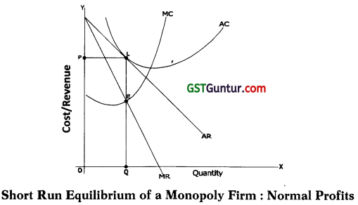
Normal Profits (AR = AC):
A firm would earn normal profits if at the equilibrium output AR=AC.

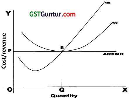
Short Run Equilibrium of a competitive firm : Normal Profits
Equilibrium point : E (MR = MC)
Equilibrium output : OQ
Average Revenue : QE (= OP)
Average Cost : QE
Therefore, AR = AC. Hence, Normal Profits.

Super Normal Profits (AR > AC):
A firm would earn super normal profits if at the equilibrium output AR > AC.

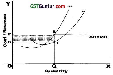
Figure : Short Run Equilibrium of a competitive firm : Super Normal Profits
Equilibrium point : E (where MR = MC)
Equilibrium output : OQ
Average Revenue : QE(= OP)
Average Cost : QF
∴ Profit Per unit : Average Revenue – Average Cost
= QE – QF = EF
Total Profits : Total output x profit per unit
= OQ X EF
Area PEFG.

Losses (AR < AC):
A firm suffer losses, if at the equilibrium level of output, its AR < AC.

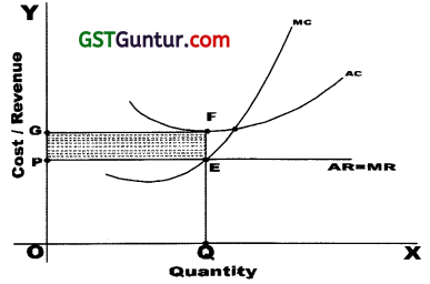
Figure : Short Run Equilibrium of Competitive Firm : Losses
Equilibrium Point : E (where MR MC)
Equilibrium Output : OQ
Average Revenue : QE
Average Cost : QF
∴ Loss per unit : Average cost – Average Revenue
= QF – QE = EF
Total Loss : Total output x loss per unit
= OQ x EF
= Area PEFG

→ When the firm incur losses, a question arises whether it should continue to produce or should it shut down ?

→ The answer to this lies in the cost structure of the firm. → Total cost of a firm = Total Fixed Costs + Total Variable Costs

→ Fixed costs once incurred cannot be recovered even if the firm shuts down.

→ Therefore, whether to shut down or not depends on variable costs alone.

→ If AR (Price) > AVC or AR = AVC, the firm can continue to produce even though it suffer losses at the equilibrium level of output.

→ If AR (Price) < AVC, the firm should shut down.

Long run Equilibrium of a Competitive Firm:
→ In a perfectly competitive market there is no restriction on the entry or exit of firms.

→ Therefore, if existing firms are earning super normal profits in the short run, they will attract new firms to enter the industry.

→ As a result of this, the supply of the commodity increases. This brings down the price per unit.

→ On the other hand, the demand for factors of productions rises which pushes up their prices and so the cost of production rises.

→ Thus, the price line or AR curve will go down and cost curves will go up.

→ As a result of this, price line or AR curve becomes tangent to long run average cost curve. This wipes out super normal profit.

→ Hence, in long run firms earn only normal profits.

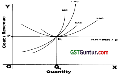
Figure : Long run equilibrium of a cofnpetitive industry and its firms.

→ Fig. Shows that long run LMR = LMC = LAC = LAR = Price

→ The firm is at equilibrium at point Er

→ E₁ is the minimum point of LAC curve. Thus firm produces equilibrium output OQ₁ at the minimum or optimum cost.

→ In the long run under competitive market –

• Firms earn just normal profits, and
• competitive firms are of optimum size because they produce at optimum cost Le. at the lowest point of long run average cost curve.

Monopoly

Introduction :
→ ‘Mono’ means single and ‘Poly’ means seller.

→ So monopoly refers to that market structure where there is a single firm producing and selling a commodity which has no close substitute.

→ As there is no rival firms producing close substitute,

• the monopoly firm itself is industry, and
• its output constitutes the total market supply.

Features of Monopoly Market:
Following are the main features of the monopoly market:
1. Single seller and Large number of buyers.

• There is only one seller or producer of a commodity in the market but there are many buyers.
• As a result, the monopoly firm has full control over the supply of the commodity.

2. No close substitutes.

• The commodity sold by the monopolist generally has no close substitutes.
• Therefore, the cross elasticity of demand between monopolist’s commodity and other commodity is zero or less than one.
• As a result monopoly firm faces a downward sloping demand curve.

3. Restrictions to entry for new firms.

• The monopoly firm controls the situation in such a way that it becomes difficult for new firms to enter the monopoly market and compete with monopoly firm.
• There are many barriers to the entry of new firm which can be economic, institutional or artificial in nature.

4. Price maker.

• A monopoly firm has full control over the supply of the commodity
• Price is solely fixed by the monopoly firm.
• So, a monopoly firm is a “price maker”.

Sources of Monopoly:
The sources of monopoly may be listed as follows :
1. Patents, copyrights and trade marks.
Legal support provided by the government to promote inventions, to produce a particular commodity, etc. by granting patents, copyrights, trademarks, etc. creates monopoly.

2. Control of raw materials.
If one firm acquires the sole ownership or control of essential raw materials, then the other firms cannot compete.

3. Economies of large scale.

• The monopoly firm may be very big and enjoy economies of large scale of production.
• The cost of production is therefore low, hence it may supply goods at low prices.
• This leaves no scope for new firms to enter the market.

4. Government control on entry:
Example – In defense production; public utility services like water, transportation, electricity, etc.

5. Business combines.
Monopolies are created by forming cartels, pools, syndicates, etc. by the firms producing the same goods to control price and output.

Average Revenue and Marginal Revenue Curves under Monopoly:

• Monopoly firm constitutes industry.
• Therefore, the entire demand of the consumers faces the monopolist
• The demand curve of a monopoly firm is the same as the market demand curve of the commodity.
• As the demand curve of the consumers for a commodity slopes downward, the monopolist faces a downward sloping demand curve.
• This means that monopolist can sell more quantity only by lowering the price of the commodity
• The demand curve facing the monopolist is also his average revenue curve. Thus, average revenue curve of the monopolist slopes downwards
• As the demand curve i.e. average revenue curve slopes downwards, marginal revenue curve will be below it.

Table : Revenue Schedule of a Monopoly Firm.

Units Sold	Price (₹) (AR)	Total Revenue ₹  (TR)	Marginal Revenue ₹ (MR)
1	10	10	10
2	9	18	8
3	8	24	6
4	7	28	4
5	6	30	2
6	5	30	0
7	4	28	-2

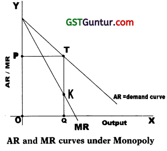
→ In the figure above, AR curve of the monopolist slopes downward and MR curve lies below it.

→ At a quantity OQ, average revenue i.e. price is OP (=QT) and marginal revenue is QK which is less than average revenue OP (=QT).

→ Thus, in case of monopoly –

• AR and MR are both negatively sloped curves,
• MR curve lies half way between the AR curve and the Y-axis,
• AR cannot be zero i.e. AR curve cannot’touch X-axis,
• MR can be zero or even negative i.e. MR curve can touch or cut the X-axis.

Short Run Equilibrium of the Monopoly Firm (Price – Output Equilibrium):
→ A monopolist will produce an output that maximizes his total profits.

→ A monopolist will maximize his total profits when –

• Marginal Cost = Marginal Revenue (MC = MR), and
• Marginal cost curve cuts the marginal revenue curve from below.

→ When a monopoly firm is in the short run equilibrium, it may find itself in the following situations –

• Firm will earn SUPER NORMAL PROFITS if its AR > AC;
• Firm will earn NORMAL PROFITS if its AR = AC, and
• Firm will suffer LOSSES if its AR < AC.

1. Super Normal Profits (AR > AC) :
The monopoly firm would earn super normal profits if at the equilibrium output AR > AC.

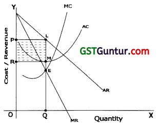
Figure : Short Run Equilibrium of a Monopoly Firm : Super Normal Profits.
Equilibrium point : E (where MR = MC)
Equilibrium output : OQ
Average Revenue : QL(= OP)
Average Cost : QM
∴ Profit Per unit : Average Revenue – Average Cost
= QL – QM = LM
Total Profits : Total Output x Profit per unit
= OQ x ML
= Area PLMR

2. Normal Profits (AR = AC) :
The monopoly firm would earn normal profits if at the equilibrium output AR = AC.

Equilibrium point : E (where MR = MC)
Equilibrium output : OQ
Average Revenue : QL
Average Cost : QL
Therefore, AR=AC.
Hence, normal profits.

3. Losses (AR < AC) :
The monopoly firm would suffer losses, if at the equilibrium output its AR < AC.

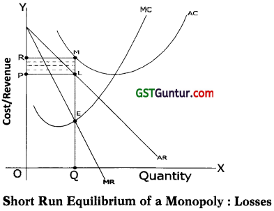
Equilibrium point : E (where MR = MC)
Equilibrium output : OQ
Average Revenue : QL(= OP)
Average Cost : QM
∴ Loss Per unit : Average Cost – Average Revenue
= QM – QL
= ML
Total Loss : Total output x Loss per unit
= OQ x ML
= Area PLMR
→ If monopoly firm’s AR > AVC or AR = AVC, it can continue to produce though it suffer losses at the equilibrium level of output.

Long Run Equilibrium of a Monopoly Firm:
→ The long run equilibrium of the monopoly firm is attained where its MARGINAL COST = MARGINAL REVENUE i.e. MC = MR.

→ The monopoly firm can continue to earn super normal profits even in the long run.

→ This is because entry to the market for new firms is blocked.

→ All costs are variable costs in the long run and these must be recovered.

→ This means that monopoly firm does not suffer loss in the long run.

→ However, if it is unable to recover variable costs, it should shut down.

→ Fig. Shows the long run equilibrium of a monopoly firm.

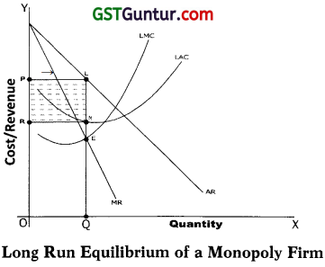
Equilibrium point : E (where MR = MC)
Equilibrium output : OQ
Average Revenue : QL(= OP)
Average Cost : QM
∴ Profit per unit : Average Cost – Average Revenue
= QL – QM = LM
Total Profits : Total Output x Profit per unit
= OQ x LM
= Area PLMR
→ Thus, we find that monopoly firm continue to earn super normal profits in long run.

→ A monopoly firm does not produce at the lowest point of LAC curve i.. does not produce at optimum level because of absence of competition.

→ In other words, it operates at sub-optimum level and therefore, does not produce optimum output.

Price Discrimination:

• A monopoly firm is also the industry.
• A single firm controls the entire supply.
• Therefore, the firm has the power to sell the same commodity to different buyers at different prices.
• When the firm charge different prices to different customers for the same commodity, it is engaged in price discrimination.
• Example – Electricity supplying firm charge higher rate per unit of electricity from industrial units than domestic consumers.

Conditions for price discrimination:
Price discrimination is possible under the following conditions :
1. Existence of two or more than two sub-markets.

• The monopolist should be able to divide the total market for his commodity into two or more sub-markets.
• Such division of market may be on the basis of income, geographic location, age, sex, etc.
• Example – on the basis of income, a doctor may charge high fees from rich patients than from poor.

2. Different markets should have different price elasticity of demand.

• The difference in price elasticity of demand in different markets enables the monopolist to discriminate among customers.
• He can charge higher price in inelastic market and lower price in elastic market.

3. No possibility of resale.

• It should not be possible for buyers to purchase the commodity from a cheaper market and sell it in the costlier markets.
• In other words, there should be no contact among the buyers of the two markets.

4. Control over supply.
The supply should be in full control of the monopolist.

Price-output determination under price discrimination:
→ Suppose a discriminating monopolist sell his output in market ‘A’ and market ‘B’.

→ Market ‘A’ has less elastic demand and market ‘B’ has more elastic demand.

→ Suppose the monopolist has only one production facility then he is faced with the questions

• How much to produce?
• How much to sell in each market?
• How much price to charge in each market?

→ The monopolist will first decide profitable level of total output (ie. where MR = MC) and then allocate the quantity between two markets.

→ The condition for equilibrium here would be –

• MC = MR_a = MR_b. It means that MC must be equal to MR in individual markets separately.
• MC = AMR (aggregate marginal revenue). It means that the monopolist must be in equilibrium not only in individual markets but also when the two markets are treated as one.

→ The process of price determination under price discrimination is shown in the following figure

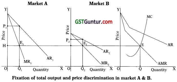
→ In the fig. – MC curve intersect the AMR curve at point E

→ Point E shows the total output is OQ.

→ When a perpendicular EH is drawn, it intersect MR_a at E₁ and MR_b at E₂. These are the equilibrium point of market A and B

→ Point E₁ shows that quantity sold in market A is OQ₁ and the price charged is OP₁.

→ Point E₂ shows that quantity sold in market B is OQ₂ and the price charged is OP₂

→ Price charged in market ‘A’ is higher than in market ‘B’.

→ Thus, a discriminating monopolist chargers a higher price in the market ‘A’ having less elastic demand and a lower price in the market ‘B’ having more elastic demand.

→ The marginal revenue is different in different markets.
Example – Suppose the single monopoly price is ₹ 40 and elasticity of demand in market A and B is 2 and 4 respectively.
MR in market A = AR_a(\(\frac { e-1 }{ e }\))
= 40(\(\frac { 2-1 }{ 2 }\))
= ₹ 20
MR in market B = AR_a(\(\frac { e-1 }{ e }\))
= 40(\(\frac { 4-1 }{ 4 }\))
= ₹ 30
→ It is clear from the above example that the marginal revenue is different in different markets when elasticity of demand at the single price is different.

→ MR is higher in the market having high elasticity and vice versa.

→ In the above example, since marginal revenue in market ‘B’ is more, it will be profitable for monopolist to transfer some units of the commodity from market ‘A’ to ‘B’.

→ When monopolist transfers the commodity from market A to B, he is practicing price discrimination.

→ As a result, the price of commodity will increase in market A and will decrease in market B.

→ Ultimately the marginal revenue in the two market will become equal.

→ When marginal revenue becomes equal in the two markets, it will no longer be profitable to transfer the units of commodity from market A to B.

Objectives of Price discrimination:
To earn maximum profit; to dispose off surplus stock; to enjoy economies of scale; to capture for¬eign markets etc.

Degrees of price discrimination:
Pigou classified price discrimination as follows:
(1) first degree price discrimination where the monopolist fix a price which take away the entire consumer’s surplus,

(2) second degree price discrimination where the monopolist take away only some part of consumer’s surplus. Here price changes according to the quantity sold.

Example – large quantity sold at a lower price, third degree price discrimination where the monopolist charges the price according to location customer segment, income level, time of purchase etc.

Imperfect competition : monopolistic competition:

Introduction:

• We have studied two models that represent the two extremes of market structures namely perfect competition and monopoly.
• The two extremes of market structures are not seen in real world.
• In reality we find only imperfect competition which fall between the two extremes of perfect competition and monopoly.
• The two main forms of imperfect competition are –
  → Monopolistic Competition and
  → Oligopoly

Meaning and features of Monopolistic Competition:

• As the name implies, monopolistic competition is a blend of competitive market and monopoly elements.
• There is competition because of large number of firms with easy entry into the industry selling similar product.
• The monopoly element is due to the fact that firms produce differentiated products. The products are similar but not identical.
• This gives an individual firm some degree of monopoly of its own differentiated product.
• Example – MIT and APTECH supply similar products, but not identical.

Similarly, bathing soaps, detergents, shoes, shampoos, tooth pastes, mineral water, fitness and health centers, ready made garments, etc. all Operate in a monopolistic competitive market.

The characteristics of monopolistic competitive market can be summed up as follows :
1. Large number of buyers and sellers
→ There are large number of firms.

• So each individual firms can not influence the market.
• Each individual firm share relatively small fraction of the total market.

→ The number of buyers is also very large and so single buyer cannot influence the market by demanding more or less.

2. Product Differentiation:

• The product produced by various firms are not identical but are somewhat different from each other but are close substitutes of each other.
• Therefore, the products are differentiated by brand names.
• Example – Colgate, Close-Up, Pepsodent, etc.
• Brand loyalty of customers gives rise to an element of monopoly to the firm.

3. Freedom of entry and exit:
New firms are free to enter into the market and existing firms are free to quit the market.

4. Non-Price Competition

• Firms under monopolistic competitive market do not compete with each other on the basis of price of product.
• They compete with each other through advertisements, better product development, better after sales services, etc.
• Thus, firms incur heavy expenditure on publicity advertisement, etc.

Short Run Equilibrium of a Firm in Monopolistic Competition. (Price-Output Equilibrium):
→ Each firm in a monopolistic competitive market is a price maker and determines the price of its own product.

→ As many close substitutes for the product are available in the market, the demand curve (average revenue curve) for the product of individual firm is relatively more elastic.

→ The conditions of equilibrium of a firm are same as they are in perfect competition and mo-nopoly ie.

• MR = MC, and
• MC curve cuts the MR curve from below.

→ The following figures show the equilibrium conditions and price-output determination of a firm under monopolistic competition.

→ When a firm in a monopolistic competition is in the short run equilibrium, it may find itself in the following situations –

• Firm will earn SUPER NORMAL PROFITS if its AR > AC;
• Firm will earn NORMAL PROFITS if its AR = AC; and
• Firm will suffer LOSSES if its AR < AC

1. Super Normal Profits (AR > AC):

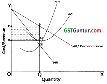
Figure : Firm’s Equilibrium under Monopolistic Competition Super Normal Profits.
Equilibrium point : E (where MR = MC)
Equilibrium output : OQ
Average Revenue : QL(= OP)
Average Cost : QM
∴ Profit per unit : Average Revenue – Average Cost
QL – QM = LM
Total Profits : Total Output x Profit per unit
= OQ X LM
= Area PLMR
The firm will earn Normal Profits if AC curve is tangent to AR curve i.e. when AR = AC

2. Losses (AR < AC):

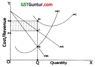
Figure : Firm’s Equilibrium under Monopolistic Competition : Losses
Equilibrium point : E (where MR = MC)
Equilibrium output : OQ
Average Revenue : QL
Average Cost : QM
∴ Loss Per unit : Average Cost – Average Revenue
= QM – QL = ML
Total Loss : Total Output x Loss per unit
= OQ x ML
= Area PLMR
The firm may continue to produce even if incurring losses if its AR ≥ AVC.

Long Run Equilibrium of a Firm in Monopolistic Competition:
→ If the firms in a monopolistic competitive market earn super normal profits, it attracts new firms to enter the industry.

→ With the entry of new firms market will be shared by more firms.

→ As a result, profits per firm will go on falling.

→ This will go on till super normal profits are wiped out and all the firms earn only normal profits.

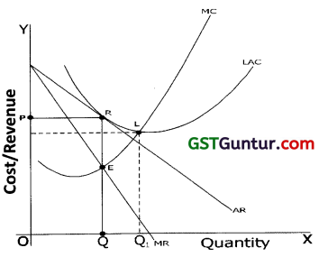
Figure : Long Run Equilibrium of a firm in Monopolistic Competition
Equilibrium Point : E(where MR = MC)
Equilibrium output : OQ
Average Revenue : QR
Average Cost : QR
Therefore, AC=AR. Hence, Normal Profits.
→ In the long run firms in a monopolistic competitive market just earn Normal profits.

→ Firms operate at sub-optimal level as shown by point ‘R’ where the falling portion AC curve is tangent to AR curve.

→ In other words firms do not operate at the minimum point of LAC curve ‘L’.

→ Therefore, production capacity equal to QQ₁, remains idle or unused called excess capacity.

→ This implies that in monopolistic competitive market –

Firms are not of optimum size and each firm has excess production capacity:

• The firm can expand its output from Q to Q₁, and reduce its average cost.
• But it will not do so because to sell more it will have to reduce its average revenue even more than average costs.
• Hence, firms will operate at sub-optimal level only in the long run.

Oligopoly

Introduction:

• ‘Oligo’ means few and ‘Poly’ means seller. Thus, oligopoly refers to the market structure where there are few sellers or firms.
• They produce and sell such goods which are either differentiated or homogeneous products.
• Oligopoly is an important form of imperfect/competition.
• Example – Cold drinks industry; automobile industry; Idea; Airtel. Hutch, BSNL mobile services in Nagpur; tea industry; etc.

Types of Oligopoly:

• Pure or perfect oligopoly occurs when the product is homogeneous in nature, Example – Aluminum industry.
• Differentiated or imperfect oligopoly where products are differentiated. Example – toilet products.
• Open oligopoly where new firms can enter the market and compete with already existing firm.
• Closed oligopoly where entry of new firm is restricted.
• Collusive oligopoly when some firms come together with some common understanding and act in collusion with each other in fixing price and output.
• Competitive oligopoly where there is no understanding or collusion among the firms.
• Partial oligopoly where the industry is dominated by one large firm which is looked upon by other firms as the leader of the group. The dominating firm will be the price leader.
• Full oligopoly where there is absence of price leadership.
• Syndicated oligopoly where the firms sell their products through a centralized syndicate.
• Organized oligopoly where the firms organize themselves into a central association for fixing prices, output, quotas, etc.

Characteristics of Oligopoly Market:
Following are the special features of oligopoly market:
1. Interdependence

• In an oligopoly market, there is interdependence among firms.
• A firm cannot take independent price and output decisions.
• This is because each firm treats other firms as rivals.
• Therefore, it has to consider the possible reaction to its rivals price-output decisions.

2. Importance of advertising and selling costs:

• Due to interdependence, the various firms have to use aggressive and defensive marketing tools to achieve larger market share.
• For this the firms spend heavily on advertisement, publicity, sales promotion, etc. to attract large number of customers.
• Firms avoid price-wars but are engaged in non-price competition. Example – free set of tea mugs with a packet of Duncan’s Double Diamond Tea.

3. Indeterminate Demand Curve:

• The nature and position of the demand curve of the oligopoly firm cannot be determined.
• This is because it cannot predict its sales correctly due to indeterminate reaction patterns of rival firms.
• Demand curve goes on shifting as rivals too change their prices in reaction to price changes by the firm.

4. Group behaviour:

• The theory of oligopoly is a theory of group behaviour.
• The members of the group may agree to pull together to promote their mutual interest or fight for individual interests or to follow the group leader or not.
• Thus the behaviour of the members is very uncertain.

Price and output decisions in an Oligopolistic Market:
→ As seen earlier, an oligopolistic firm does not know how rival firms react to each other decisions. Therefore, it has to be very careful when it makes decision about its price. Rival firms retaliate to price change by an oligopolistic firm.

Hence, its demand curve indeterminate. Price and output cannot be fixed. Some of the important oligopoly models are:
1. Some economists assume that oligopolistic firms make their decisions independently. Therefore, the demand curve becomes definite and hence equilibrium level of output can be determined.

2. Some believe that oligopolistic can predict the reaction of rivals on the basis of which he makes decisions about price and quantity.

3. Cornet considers OUTPUT is the firm’s controlled variable and not price.

4. In a model given by Stackelberg, the leader firm commits to an output before all other firms. The rest of firms follow it and choose their own level of output.

5. Bertrand model states PRICE is the control variable for firms and therefore each firm sets the price independently.

6. In order to pursue common interests, oligopolistic enter into enter into agreement and jointly act as monopoly to fix quantity and price.

Price Leadership:
→ A large or dominant firm may be surrounded by many small firms. The dominant firm takes the lead to set the price taking into account of the small firms. Dominant firm may adopt any one of the following strategies –
1. ‘Live and let live’ strategy where dominant firm accepts the presence of small firms and set the price. This is called price-leadership,

2. In another strategy, the price leader sets the price in such a way that it allows some profits to the follower firms.

3. Barometric price leadership where an old, experienced, respectful, largest acts as a leader and sets the price. It makes changes in price which are beneficial from all firm’s and industry’s view point. Price charged by leader is accepted by follower firms.

Kinked Demand Curve :
→ In many oligopolistic industries there is price rigidity or stability.

→ The prices remains sticky or inflexible for a long time.

→ Oligopolists do not change the price even if economic conditions change.

→ Out of many theories explaining price rigidity, the theory of kinked demand curve hypothesis given by American economist Paul M. Sweezy is most popular.

→ According to kinked demand curve 4 hypothesis, the demand curve faced by an oligopolist have a ‘Kink’ at the prevailing price level.

→ A kink is formed at the prevailing price because –

• the portion of the demand curve above the prevailing price is elastic, and
• the portion of the demand curve below the prevailing price is inelastic

→ Consider the following figure.

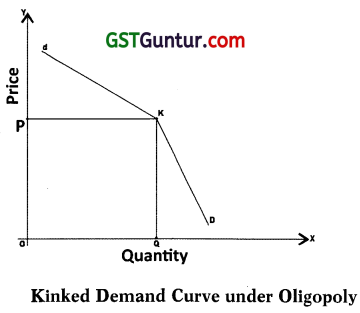
→ In the fig., OP is the prevailing price at which the firm is producing and selling OQ output.

→ At prevailing price OP, the upper portion of demand curve dK is elastic and lower portion of demand curve KD is inelastic.

→ This difference in elasticities is due to the assumption of particular reactions by kinked demand curve theory.

→ The assumed reaction pattern are –
1. If the oligopolist raises the price above the prevailing price OP, he fears that none of his rivals will follow him.

• Therefore, he will loose customers to them and there will be substantial fall in his sales.
• Thus, the demand with respect to price rise above the prevailing price is highly elastic as indicated by the upper portion of demand curve dK.
• The oligopolist will therefore, stick to the prevailing prices.

2. If the oligopolist reduces the price below the prevailing price OP to increase his sales, his rivals too will quickly reduce the price.

• This is because the rivals fear that their customers will get diverted to price cutting oligopolist’s product.
• Thus, the price cutting oligopolist will not be able to increase his sales very much.
• Hence, the demand with respect to price reduction below the prevailing price is inelastic as indicated by the lower portion of demand curve KD.
• The oligopolist will therefore, stick to the prevailing prices.
• Each oligopolist will, thus, stick to the prevailing price realising no gain in changing the price.
• A kink will, therefore, be formed at the prevailing price which remains rigid or sticky or stable at this level.

Other Important Market Forms:

• Duopoly in which there are only TWO firms in the market. It is subset of oligopoly.
• Monopoly is a market where there is a single buyer. It is generally in factor market.
• Oligopsony market where there are small number of large buyers in factor market.
• Bilateral monopoly market where there is a single buyer and a single seller.
• It is mix of monopoly and monopsony markets.