Theory of Demand and Supply – CA Foundation Economics Notes Chapter 2

Browsing through CA Foundation Business Economics Notes Chapter 2 Theory of Demand and Supply help students to revise the complete subject quickly.

Theory of Demand and Supply – Business Economics CA Foundation Notes Chapter 2

Meaning of Demand:

In ordinary speech, the term demand is many times confused with ‘desire’ or ‘want’.
Desire is only a wish to have any thing.
In economics demand means more than mere desire.
Demand in economics means an effective desire for a commodity i.e. desire backed by the ‘ability to pay’ and ‘willingness to pay’ for it.
Thus, demand refers to the quantity of a good or service that consumers are willing and able to purchase at different prices during a period of time.
Thus, defined, the term demand shows the following features:
→ Demand is always with reference to a PRICE.
→ Demand is to be referred to IN A GIVEN PERIOD OF TIME.
→ Consumer must have the necessary purchasing power to back his desire for the commodity.
→ Consumer must also be ready to exchange his money for the commodity he desires.
Example: Mr. A’s demand for sugar at ₹ 15 per kg. is 4 kgs. per week.

Determinants of Demand:
For estimating market demand for its products, a firm must have knowledge about –

the determinants of demand for its product, and
the nature of relationship between demand and is determinants.

The various factors on which the demand for a product/commodity depends are as follows:

Price of the commodity:

Other things being equal, the demand for a commodity is inversely related with its price.
It means that a rise in price of a commodity brings about fall in its demand and vice versa.
This happens because of income and substitution effects.

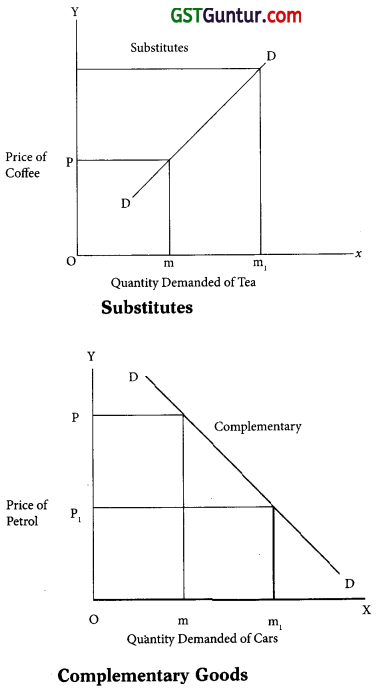
Price of the related commodities:

The demand for a commodity also depends on the prices of related commodities.
Related commodities are of two types namely –
→ Substitutes or competitive goods, &
→ Complementary goods.
Substitute goods are those goods which can be used with equal ease in place of one another.
Example – Essar Speed Card and Airtel Magic Card; Coke and Pepsi; ball pen and ink pen; tea and coffee; etc.
Demand for a particular commodity is affected if the price of its substitute falls or rises.
Example – If the price of Airtel Magic card falls, its demand will increase and demand for Essar Speed Card would fall and vice versa.
Thus, there is a POSITIVE RELATIONSHIP between price of a commodity and demand for its substitutes.
Complementary good are those goods whose utility depends upon the availability of both the goods as both are to be used together.
Example – a ball pen and refill; car and petrol; a hand set and phone connection; a tonga and horse, etc.
The demand for complementary goods have an INVERSE RELATIONSHIP with the price of related goods.
Example – If the price of Scooters falls, its demand will increase leading to increase in demand for petrol.

Income of the consumers:
1. Other things being equal, generally the quantity demanded of a commodity bear a DIRECT RELATIONSHIP to the income of the consumer i.e. with an increase in income, the demand for a commodity rises.

2. However, this may not always hold true. It depends upon the class to which commodity belongs i.e. necessaries or comforts and luxuries or inferior goods:
→ Necessaries (E.g. Food, clothing and shelter). Initially, with an increase in the in-come, the demand for necessaries also rises upto some limit. Beyond that limit, an increase in income will leave the demand unaffected.

→ Comforts and Luxurious (Example Car; Air-Conditioners; etc.) Quantity demanded of these group of commodities have a DIRECT RELATIONSHIP with the income of the consumers. As the income increases, the demand for comforts and luxuries also increases.

→ Inferior goods (E.g. Coarse grain; rough cloth; skimmed milk; etc.). Inferior goods are those goods for which superior substitutes are available Quantity demanded of this group of commodities Have an INVERSE RELATIONSHIP with the income of the consumer. E.g. A consumer starts consuming full cream milk (normal good) in place of toned milk (inferior good) with an increase in income.

Therefore, it is essential that business managers must know –

the nature of good they produce,
the nature of relationship between the quantities demanded and changes in consumer’s income, and
the factors that could bring about changes in the incomes of the consumers.

Tastes and Preferences of the consumers:
1. Tastes and preferences of consumers generally change over time due to fashion, advertisements, habits, age, family composition, etc. Demand for a commodity bears a direct relationship to those determinants.

2. Modern goods or fashionable goods have more demand than the goods which are of old design and out of fashion. Example: People are discarding Bajaj Scooter for say Activa Scooter.

3. The demand of certain goods is determined by ‘bandwagon effect’ or ‘demonstration effect’. It means a buyer wants to have a good because others have it. It means that an individual consumer’s demand is conditioned by the consumption of others.

4. Taste and preferences may also undergo a change when consumer discover that con-sumption of a good increases his PRESTIGE. Example:Diamonds, fancy cars, etc.

5. A good loses its prestige when it becomes a commonly used good. This is called ‘snob effect’.

6. Status seeking rich people buy highly priced goods only. This form of ‘conspicuous consumption’ or ‘ostentatius consumption’ is called ‘VEBLEN EFFECT’ (named after American economist THORSTEIN VEBLEN)

7. Tastes and preferences of people change either due to external causes or internal causes.

8. Therefore, knowledge about tastes and preferences is important in production planning, designing new products and services to suit the changing tastes and preferences of the consumers.

Other Factors. Other things being equal demand for a commodity is also determined by the following factors:
1. Size and composition of Population:

Generally, larger the size of population of a country, more will be the demand of the commodities.
The composition of the population also determines the demand for various commodities.
Example: If the number of teenagers is large, the demand for trendy clothes, shoes, movies, etc. will be high.

2. The level of National Income and its Distribution:

National Income is an important determinant of market demand. Higher the national income, higher will be the demand for normal goods and services.
If the income in a country is unevenly distributed, the demand for consumer goods will be less.
If the income is evenly distributed, there is higher demand for consumer goods.

3. Sociological factors:
The household’s demand for goods also depends upon sociological factors like class, family background, education, marital status, age, locality, etc.

4. Weather conditions:

Changes in weather conditions also influence household’s demand.
Example: Extraordinary hot summer push up the demand for ice-creams, cold drinks, coolers etc.

5. Advertisement:

A clever and continuous campaign and advertisement create a new type of demand.
Example: Toilet products like soaps, tooth pastes, creams etc.

6. Government Policy:

The government’s taxation policy also affects the demand for commodities.
High tax on a commodity will lead to fall in the demand of the commodity.

7. Expectation about future prices:
If consumers expect rise in the price of a commodity in near future, the current demand for the commodity will increase and vice versa,

8. Trade Conditions:

If the country is passing through boom conditions, demand for most goods is more.
But during depression condition, the level of demand falls.

9. Consumer-credit facility and interest rates:
If ample credit facilities with low rates of interest is available, there will be more demand specially of consumer durable goods like scooters, LCD /LED televisions, refrigerators, home theatre, etc.

Demand Function:
1. Mathematical/symbolic statement of functional relationship between the demand for a product (the dependent variable) its determinants (the independent variables) is called demand function
D_x = f (P_x, M, P_s ; P_c, T, A)
Where –
D_x = quantity demanded of product X
P_x = the price of the product X
M = money income of the consumer
P_s = the price of its substitute
P_c = the price of its complementary goods
T = consumer’s tastes and preferences
A = advertising effect measured through the level of advertisement expenditure.

The Law of Demand:
→ The Law of Demand expresses the nature of functional relationship between the price of a commodity and its quantity demanded.

→ It simply states that demand varies inversely to the changes in price i.e. demand for a com-modity expands when price falls and contracts when price rises.

→ “Law of Demand states that people will buy more at lower prices and buy less at higher prices, other things remaining the same.” (Prof. Samuelson)

→ It is assumed that other determinants of demand are constant and ONLY PRICE IS THE VARIABLE AND INFLUENCING FACTOR.

→ Thus, the law of demand is based on the following main assumptions:

Consumers income remain unchanged.
Tastes and preferences of consumers remain unchanged.
Price of substitute goods and complement goods remain unchanged.
There are no expectations of future changes in the price of the commodity.
There is no change in the fashion of the commodity etc.

→ The law can be explained with the help of a demand schedule and a corresponding demand curve.

→ Demand schedule is a table or a chart which shows the different quantities of commodity demanded at different prices in a given period of time.

→ Demand schedule can be Individual Demand Schedule or Market Demand Schedule.

→ Individual Demand Schedule is a table showing different quantities of commodity that ONE PARTICULAR CONSUMER is willing to buy at different level of prices, during a given period of time.
Table 1 : Demand Scheduled of an Individual Buyer:

Price of sugur ₹ per kg.	Quantity Demanded kgs.per month
1	5
2	4
3	3
4	2
5	1

Table 2 : Market Demand Schedule

Price of sugar ₹ per kg.	Quantity Demanded p.m. kgs		Market Demand A + B
Price of sugar ₹ per kg.	Consumer A	Consumer B	Market Demand A + B
1	5	6	5 + 6 = 11
2	4	5	4 + 5 = 9
3	3	4	3 + 4 = 7
4	2	3	2 + 3 = 5
5	1	2	1 + 2 = 3

(Assumption: There are only 2 buyers in the market)
→ Both individual and market schedules denotes an INVERSE functional relationship between price and quantity demanded. In other words, when price rises demand tends to fall and vice versa.

A demand curve is a graphical representation of a demand schedule or demand function.
→ A demand curve for any commodity can be drawn by plotting each combination of price and demand on a graph.

→ Price (independent variable) is taken on the Y-axis and quantity demanded (dependent variable) on the X-axis.

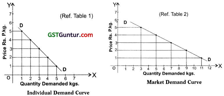
→ Individual Demand Curve as well as Market Demand Curve slope downward from left to right indicating an inverse relationship between own price of the commodity and its quantity demanded.

→ Market Demand Curve is flatter than individual Demand Curve.

→ Reasons for the law of demand and downward slope of a demand curve are as follows:
1. The Law of Diminishing Marginal Utility:

According to this law, other things being equal as we consume a commodity, the marginal utility derived from its successive units go on falling.
Hence, the consumer purchases more units only at a lower price.
A consumer goes on purchasing a commodity till the marginal utility of the commodity is greater than its market price and stops when MU = Price i.e. when consumer is at equilibrium.
When the price of the commodity falls, MU of the commodity becomes greater than price and so consumer start purchasing more till again MU = Price.
It therefore, follows that the diminishing marginal utility implies downward sloping demand curve and the law of demand operates.

2. Change in the number of consumers:

Many consumers who were unable to buy a commodity at higher price also start buying when the price of the commodity falls.
Old customers starts buying more when price falls.

3. Various uses of a commodity:
Commodity may have many uses. The number of uses to which the commodity can be put will increase at a lower price and vice versa.

4. Income effect:

When price of a commodity falls, the purchasing power (i.e. the real income) of the consumer increases.
Thus he can purchase the same quantity with lesser money or he can get more quantity for the same money.
This is called income effect of the change in price of the commodity.

5. Substitution effect:

When price of a commodity falls it becomes relatively cheaper than other commodities.
As a result the consumer would like to substitute it for other commodities which have now become more expensive. Example: With the fall in price of tea, coffee’s price remaining the same, tea will be substituted for coffee.
This is called substitution effect of the change in price of the commodity.
Thus, Price effect = Income Effect + Substitution Effect as Explained by Hicks and Allen.

Exceptions to the Law of Demand:
→ Law of Demand expresses the inverse relationship between price and quantity demanded of a commodity. It is generally valid in most of the situations.

→ But, there are some situations under which there may be direct relationship between price and quantity demanded of a commodity.

→ These are known as exceptions to the law of demand and are as follows:
1. Giffen Goods:

In some cases, demand for a commodity falls when its price fall and vice versa.
In case of inferior goods like jawar, bajra, cheap bread, etc. also called “Giffen Goods” (known after its discoverer Sir Robert Giffens) demand is of this nature.
When the price of such inferior goods fall, less quantity is purchased due consumer’s increased preference for superior commodity with the rise in their “real income” (i.e. purchasing power).
Hence, other things being equal, if price of a Giffen good fall its demand also falls.
There is positive price effect in this case.

2. Conspicuous goods:

Some consumers measure utility of a commodity by its price i.e. if the commodity is expensive they think it has got more utility and vice versa.
Therefore, they buy less at lower price and more of it at higher price. Example: Diamonds, fancy cars, dinning at 5 stars, high priced shoes, ties, etc….
Higher prices are indicators of higher utilities.
A higher price means higher prestige value and higher appeal and vice versa.
Thus a fall in their price would lead to fall in their quantities demanded. This is against the law of demand.
This was found out by Veblen in his doctrine of “Conspicuous Consumption” and hence this effect is called Vebleri effect or prestige effect.

3. Conspicuous necessities:

The demand for some goods is guided by the demonstration effect of the consumption pattern of a social group to which the person belongs.
Example – Television sets, refrigerators, music systems, cars, fancy clothes, washing machines etc.
Such goods are used just to demonstrate that the person is not inferior to others in group.
Hence, inspite of the fact that prices have been continuously rising, their demand does not show tendency to fall.

4. Future changes in prices:
When the prices are rising, households tend to purchase larger quantities of the commodity, out of fear that prices may go up further and vice versa. Example – Shares of a good company, etc.

5. Irrational behaviour of the consumers:
At times consumers make IMPULSIVE PURCHASES without any calculation about price and usefulness of the product. In such cases the law of demand fails.

6. Ignorance effect:
Many times households may demand larger quantity of a commodity even at a higher price because of ignorance about the ruling price of the commodity in the market.

7. Consumer’s illusion:

Many consumers have a wrong illusion that the quality of the commodity also changes with the price change.
A consumer may contract his demand with a fall in price and vice versa.

8. Demand for necessaries:
The law of demand does not hold true in case of commodities which are necessities of life. Whatever may be the price changes, people have to consume the minimum quantities of necessary commodities. Example – rice, wheat, clothes, medicines, etc.

Expansion and Contraction of Demand (changes in quantity demanded. Or movement along a demand curve):
→ The law of demand, the demand schedule and the demand curve all show that

when the price of a commodity falls its quantity demanded rises or expansion takes place and
when the price of a commodity rises its quantity demanded fall or contraction takes place.

→ Thus, expansion and contraction of demand means changes in quantity demanded due to change in the price of the commodity other determinants like income, tastes, etc. remaining constant or unchanged.

→ When price of a commodity falls, its quantity demanded rises. This is called expansion of demand.

→ When price of a commodity rises, its quantity demanded falls. This is called contraction of demand.

→ As other determinants of price like income, tastes, price of related goods etc. are constant, the position of the demand curve remains the same. The consumer will move upwards or downwards on the same demand curve.

In the figure
→ At price OP quantity demanded is OQ.

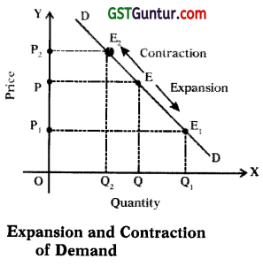
→ With a fall in price to OP₁, the quantity demanded rises from OQ to OQ₁. The coordinate point moves down from E to E₁. This is called ‘expansion of demand’ or ‘a rise in quantity demanded’ or ‘downward movement on the same demand curve’.

→ At price OP quantity demanded is OQ.

→ With a rise in price to P₂, the quantity demanded falls from OQ to OQ₂. The coordinate point moves up from E to E₂. This is called ‘contraction of demand’ or ‘a fall in quantity demanded’ or ‘upward movement on the same demand curve’.

→ Thus, the downward movement on demand curve is known as expansion in demand and an upward movement on demand curve is known as contraction of demand.

Increase and Decrease in demand (changes in demand OR shift in demand curve):
1. When there is change in demand due to change in factors other than price of the commodity, it is called increase or decrease in demand.

2. It is the result of change in consumer’s income, tastes and preferences, changes in population, changes in the distribution of income, etc.

3. Thus, price remaining the same when demand rises due to change in factors other than price, it is called increase in demand. Here, more quantity is purchased at same price or same quantity is purchased at higher price.

4. Likewise price remaining the same when demand falls due to change in factors other than price, it is called decrease in demand. Here, less quantity is purchased at ame price or same quantity is purchased at lower price.

5. In above cases demand curve shifts from its original position to rightward when demand increases and to leftward when demand decreases. Thus, change in demand curve as a result of increase or decrease in demand, is technically called shift in demand curve.

In the figure
1. Original demand curve is DD. At OP price OQ quantity is being demanded.

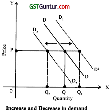
2. As the demand changes, the demand curve shifts either to the right (D₁D₁) or to the left (D₂D₂)

3. At D₁D₁, OQ₁ quantity is being demanded at the price OP. This shows increase in demand (rightward shifts in demand curve) due to factor other than price.

4. At D₂D₂, QO₂ quantity is being demanded at the price OP. This shows decrease in demand (leftward shift in demand curve) due to a factor other than price.

5. When demand of a commodity INCREASES due to factors other than price, firms can sell a larger quantity at the prevailing price and earn higher revenue.

6. The aim of a advertisement and sales promotion activities is to shift the demand curve to the right and to reduce the elasticity of demand.

Elasticity of Demand:

Elasticity of demand is defined as the responsiveness or sensitiveness of the quantity demanded of a commodity to the changes in any one of the variables on which demand depends.
These variables are price of the commodity, prices of the related commodities, income of the consumers and many other factors on which demand depends.
Accordingly, we have price elasticity, cross elasticity, elasticity of substitution, income elasticity and advertisement elasticity.
Unless mentioned otherwise, it is price elasticity of demand which is generally referred.

Price Elasticity of Demand:
→ Price elasticity measures the degree of responsiveness of quantity demanded of a commodity to a change in its price, given the consumer’s income, his tastes and prices of all other goods.

→ It reflects how sensitive buyers are to change in price.

→ Price elasticity of demand can be defined “as a ratio of the percentage change in the quantity demanded of a commodity to the percentage change in its own price”.

→ It may be expressed as follows:

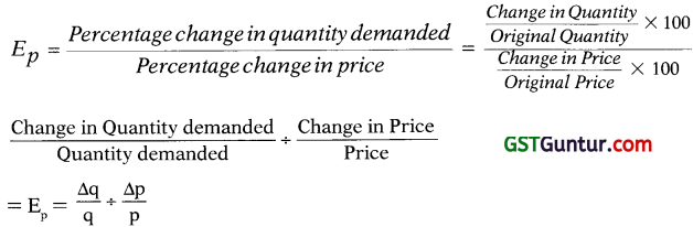
→ Rearranging the above expression we get:
E_p = \(\frac{\Delta q}{q} \times \frac{p}{\Delta p}=\frac{\Delta q}{\Delta p} \times \frac{p}{q}\)
Where –
q = Original quantity demanded
p = Original price
∆ = indicates change
E = price elasticity

→ Since price and quantity demanded are inversely related, the value of price elasticity coefficient will always be negative. But for the value of elasticity coefficients we ignore the negative sign and consider the numerical value only.

→ The value of elasticity coefficients will vary from zero to infinity.

When the coefficient is zero, demand is said to be perfectly inelastic.
When the coefficient lies between zero and unity, demand is said to be inelastic.
When coefficient is equal to unity, demand has unit elasticity.
When coefficient is greater than one, demand is said to elastic.
In extreme cases co-efficient could be infinite.

The degrees (types) of price elasticity of demand.
→ Price elasticity measures the degree of responsiveness of quantity demanded of a commodity to a change in its price. Depending upon the degree of responsiveness of the quantity demanded to the price changes, we can have the following kinds of price elasticity of demand.
1. Perfectly Inelastic Demand: (E_p = 0):

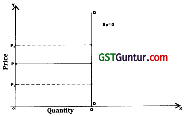
When change in price has no effect on quantity demanded, then demand is perfectly inelastic. Example – If price falls by 20% and the quantity demanded remains unchanged then, E_p = \(\frac { 0 }{ 20 }\) = 0. In this case, the demand curve is a vertical straight line curve parallel to y-axis as shown in the figure.

2. Perfectly Elastic Demand: (E_p = ∞):

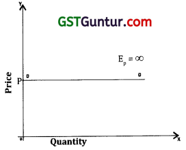
When with no change in price or with very little change in price, the demand for a commodity expands or contracts to any extent, the demand is said to be perfectly elastic. In this case, the demand curve is a horizontal and parallel to X-axis. The figure shows that demand curve DD is parallel to X-axis which means that at given price, demand is ever increasing.

3. Unit Elastic Demand: (E_p = 1):

When the percentage or proportionate change in price is equal to the percentage or proportionate change in quantity demanded, then the demand is said to be unit elastic.
Example: If price falls by 10% and the demand rises by 10% then, Demand Curve DD is a rectangular hyperbola curve suggesting unitary elastic demand.

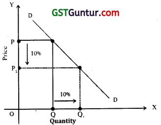
4. Relatively Elastic Demand: ( E_p > 1):
When a small change in price leads to more than proportionate change in quantity demanded then the demand is said to be relatively elastic
Example: If price falls by 10% and demand rises to by 30% then, E_p = \(\frac { 30 }{ 10 }\) = 3 > 1. The coefficient of price elasticity would be somewhere between ONE and INFINITY. The elastic demand curve is flatter as shown in figure.

Demand curve DD is flat suggesting that the demand is relatively elastic or highly elastic. Relatively elastic demand occurs in case of less urgent wants or if the expenditure on commodity is large or if close substitutes are available.

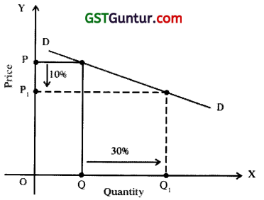
5. Relatively Inelastic Demand: (E_p < 1):
When a big change in price leads to less than proportionate change in quantity demanded, then the demand is said to be relatively inelastic.

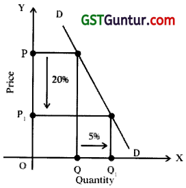
Example: If price falls by 20% and demand rises by 5% then, E_p = \(\frac { 5 }{ 20 }\) = \(\frac { 1 }{ 4 }\) < 1 The coefficient of price elasticity is somewhere between ZERO and ONE. The demand curve in this case has steep slope.
Demand curve DD is steeper suggesting that demand is less elastic or relatively inelastic. Relatively inelastic demand occurs in case compulsory goods i.e. necessities of life.

Measurement of price elasticity of demand:
The different methods of measuring price elasticity of demand are:

The Percentage or Ratio or Proportional Method,
The Total Outlay Method,
The Point or Geometrical Method, and
The Arc Method.

1. The Percentage Method:
This method is based on the definition of elasticity of demand. The coefficient of price elasticity of demand is measured by taking ratio of percentage change in demand to the percentage change in price. Thus, we measure the price elasticity by using the following formula –
E_p = \(\frac { ∆q }{ q }\) x \(\frac { p }{ ∆q }\) = \(\frac { ∆q }{ ∆p }\) x \(\frac { p }{ q }\)
Where –
∆ q = Change in quantity demanded
q = Original quantity demanded
∆ p = change in price
p = Original price
If the coefficient of above ratio is equal to ONE or UNITY, the demand will be unitary.
If the coefficient of above ratio is MORE THAN ONE, the demand is relatively elastic.
If the coefficient of above ratio is LESS THAN ONE, the demand is relatively inelastic.

2. The Total Outlay or Expenditure Method or Seller’s Total Revenue Method:
The total outlay refers to the total expenditure done by a consumer on the purchase of a commodity. It is obtained by multiplying the price with the quantity demanded. Thus,
Total Outlay (TO) = Price (P) X Quantity (Q)
TO = P X Q
In this method, we measure price elasticity by examining the change in total outlay due to change in price.
Dr. Alfred Marshall laid the following propositions:

When with the change in price, the TO remains unchanged, E_p = 1.
When with a rise in price, the TO falls or with a fall in price, the TO rises, E_p > 1.
When with a rise in price, the TO also rises and with a fall in price, the TO also falls, E_p < 1.

Price per Unit (₹)	Quantity Demanded	Total Outlay (P x Q)	Elasticity of Demand
5 4	20 Units 25 Units	100 100	E_p = 1 Unitary
5 4	20 Units 25 Units	100 120	E_p > 1 Elastic
5 4	20 Units 25 Units	100 88	E_p < 1 Inelastic

→ However, total outlay method of measuring price elasticity is less exact. This method only classifies elasticity into elastic, inelastic and unit elastic.

→ The exact and precise coefficient of elasticity cannot be found out with this method.

3. The Point Method or Geometric Method:
→ The point elasticity method, we measure elasticity at a given point on a demand curve.

→ This method is useful when changes in price and quantity demanded are very small so that they can be considered one and the* same point only.

→ Example: If price of X commodity was ₹ 5,000 per unit and now it changes to ₹ 5002 per unit which is very small change. In such a situation we measure elasticity at a point on demand curve by using formula \(\frac { ∆q }{ ∆p }\) x \(\frac { p }{ q }\)

→ Diagrammatically also we can find elasticity at a point by using the formula –

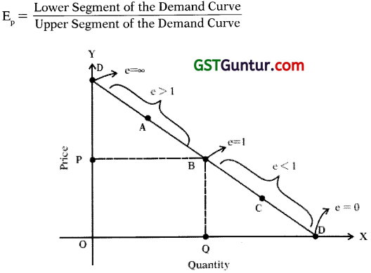
Figure:

The figure shows that even though the shape of the demand curve is constant, the elasticity is different at different points on the curve.
If the demand curve is not a straight line curve, then in order to measure elasticity at a point on demand curve we have to draw tangent at the given point and then measure elasticity using the above formula.
We can also find out numerical elasticities on different points.

4. The Arc Elasticity Method:
→ When there is large change in the price or we have to measure elasticity over an arc of the demand curve, we use the “arc method” to measure price elasticity of demand.

→ The arc elasticity is a measure of the “average elasticity” ie. elasticity at MID-POINT that connects the two points on the demand curve.

→ Thus, an arc is a portion of a curved line, hence a portion of a demand curve. Here instead of using original or new data as the basis of measurement, we use average of the two.

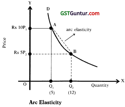
→ The formula used is –
E_p = \(\frac{\mathrm{q}_{1}-\mathrm{q}_{2}}{\mathrm{q}_{1}+\mathrm{q}_{2}} \times \frac{\mathrm{p}_{1}+\mathrm{p}_{2}}{\mathrm{p}_{1}-\mathrm{p}_{2}}\)
Where – P₁ & q₁ = Original price and quantity
p₂ & q₂ = new price and quantity
E_p = \(\frac{5-12}{5+12} \times \frac{10+5}{10-5}\)
E_p = \(\frac{-7}{17} \times \frac{15}{5}\) = E_p = \(\frac { 21 }{ 17 }\) = 1.23
E_p = 1.23

Determinants of price elasticity of demand:
Price elasticity of demand which measures the degree of responsiveness of quantity demand¬ed of a commodity to a change in price (other things remaining unchanged) depends on the following factors –
1. Nature of commodity:

The demand for necessities of life like food, clothing, housing etc. is less elastic or inelastic because people have to buy them whatever be the price.
Whereas, demand for luxury goods like cars, air-conditioners, cellular phone, etc. is elastic.

2. Availability of Substitutes:

If for a commodity wide range of close substitutes are available i.e. if a commodity is easily replaceable by others, its demand is relatively elastic. Example – Demand for cold drinks like Thumbs-up, Coca-cola, Limca, etc.
Conversely, a commodity having no close substitute has inelastic demand. Example – Salt (but demand for TATA BRAND SALT is elastic.)

3. Number of uses of a commodity:

A commodity which has many uses will have relatively elastic demand.
Example – Electricity can be put to many uses like lighting, cooking, motive-power, etc. If the price of electricity falls, its consumption for various purposes will rise and vice versa.
On the other hand if a commodity has limited uses will have inelastic demand.

4. Price range:

If price of a commodity is either too high or too low, its demand is inelastic but those which are in middle price range have elastic demand.

5. Position of a commodity in the budget of consumer:

If a consumer spends a small proportion of his income to purchase a commodity, the demand is inelastic.
Example – Newspaper, match box, salt, buttons, needles.
But if consumer spends a large proportion of his income to purchase a commodity, the demand is elastic.
Example -Clothes, milk, etc.

6. Time period:

The longer any price change remains the greater is the price elasticity of demand.
On the other hand, shorter any price change remains, the lesser is the price elasticity of demand.

7. Habits:

Habits makes the demand for a commodity relatively inelastic.
Example – A smoker’s demand for cigarettes tend to be relatively inelastic even at higher price.

8. Tied Demand (Joint Demand):

Some goods are demanded because they are used jointly with other goods. Such goods normally have inelastic demand as against goods having autonomous demand.
Example – Printers & Cartridges.

Knowledge of the concept of elasticity of demand and the factors that may change it is of great IMPORTANCE in practical life. The concept of elasticity of demand is helpful to –
1. Business Managers as it helps then to recognise the effect of price change on their total sales and revenues. The objective of a firm is profit maximization. If demand is ELASTIC for the product, the managers can fix a lower price in order to expand the volume of sales and vice versa.

2. Government for determining the prices of goods and services provided by them.

Example 1 : transport, electricity, water, cooking gas, etc. It also helps governments to understand the nature of response of demand when taxes are raised and its effect on the tax revenues.
Example 2 : Higher taxes are imposed on the goods having INELASTIC DEMAND like cigarettes, liquor, etc.

Income Elasticity of Demand:
→ The income elasticity of demand measures the degree of responsiveness of quantity demanded to changes in income of the consumers.

→ The income elasticity is defined as a ratio of percentage change in the quantity demanded to the percentage change in income.

Symbolically – E_y = \(\frac { ∆Q }{ ∆Y }\) x \(\frac { Y }{ Q }\)
Where – AQ &AY denote new quantity & income.
Q & Y denote original quantity & income.

The income elasticity of demand is Positive for all normal or luxury goods and the income elasticity of demand is Negative for inferior goods. Income elasticity can be classified under five heads:
1. Zero Income Elasticity:

It means that a given increase in income does not at all lead to any increase in quantity demanded of the commodity.
In other words, demand for the commodity is completely income inelastic or E_y < 0.
Commodities having zero income elasticity are called Neutral Goods.
Example – Demand in case of Salt, Match Box, Kerosene Oil, Post Cards, etc.

2. Negative Income Elasticity;

It means that an increase in income results in fall in the quantity demanded of the commodity or E_y <0.
Commodities having negative income elasticity are called Inferior Goods. Example – Jawar, Bajra, etc.

3. Unitary Income Elasticity:

It means that the proportion of consumer’s income spent on the commodity remains unchanged before and after the increase in income or E_y = 1. This represents a useful dividing line.

4. Income Elasticity Greater Than Unity:

It refers to a situation where the consumers spends Greater proportion of his income on a commodity when he becomes richer. E_y > 1,
Example – In the case of Luxuries like cars, T.V. sets, music system, etc.

5. Income Elasticity Less Than Unity:
It refers to a situation where the consumer spends a Smaller proportion of his income on a commodity when he becomes richer. E_y < 1,

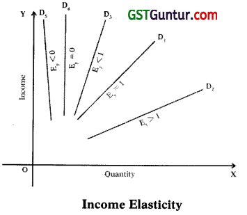
Example – In the case of Necessities like rice, wheat, etc.

Cross elasticity of demand:
→ Many times demand for two goods are related to each other.

→ Therefore, when the price of a particular commodity changes, the demand for other com¬modities changes, even though their own prices have not changed.

→ We measures this change under cross elasticity.

→ The cross elasticity of demand can be defined “as the degree of responsiveness of demand for a commodity to a given change in the price of some RELATED commodity” OR “as the ratio of percentage change in quantity demanded of commodity X to a given percentage change in the price of the related commodity Y”. Symbolically:
E_c = \(\frac { % Change in demand of X }{ % Change in the price of Y }\)
E_c = \(\frac{\Delta \mathrm{qx}}{\Delta \mathrm{py}} \times \frac{\mathrm{py}}{\mathrm{qx}}\)
Where E_c = cross elasticity
qx = Original quantity of X which is demanded
py = Original price of Y
∆ = denotes change

→ Cross elasticity of demand can be used to classify goods as follows:
1. Substitute Goods:
Example: Tea and Coffee. The cross elasticity between two substitutes is always Positive. If cross elasticity is infinite, the two goods are perfect substitute and if it is greater than zero but less than infinity, the goods are substitutes.

2. Independent Goods:
Example: Pastry and Scooter. The two commodities are not related. The cross elasticity in such cases is Zero.

3. Complementary Goods:
Example: Petrol and Car. If the price of petrol rise, its demand falls and along with it demand for cars also falls. The cross elasticity in such cases is Negative.

Advertisement or Promotional Elasticity of Demand:
→ Demand of many goods is also influenced by advertisement or promotional efforts.

→ It means that the demand for a good is responsive to the advertisement expenditure incurred by a firm.

→ The measurement of the degree of responsiveness of demand of a good to a given change in advertisement expenditure is called advertisement or promotional elasticity of demand.

→ It measures the percentage change in demand to a give ONE PERCENTAGE change in advertising expenditure. It helps a firm to know the effectiveness of its advertisement campaign.

→ Advertisement elasticity of demand is POSITIVE. Higher the value, higher is change in demand to change in advertisement expenditure.
E_a = \(\frac { % Change in demand of X }{ % Change in the Advertisement Expenditure }\)
E_a = \(\frac{\Delta Q}{\Delta A} \times \frac{A}{Q}\)
Where –
A = advertisement expenditure
Q = quantity demanded
∆ = change

→ The value of advertisement elasticity varies between zero and infinity. If –

E_a = 0, no change in demand to increase in advertisement expenditure
E_a > 0 but < 1, less than proportionate change in demand to a change in advertisement expenditure
E_a = 1, change in demand is equal to change in advertisement expenditure
E_a > 1, higher rate of change in demand than change in advertisement expenditure

Demand Forecasting

Meaning:

Demand forecasting is an estimate of the future market demand for a product. The process of forecasting is based on reliable statistical data of past and present behaviour, trends, etc.
Demand forecasting cannot be hundred per cent correct. But, it gives a reliable estimates of the possible outcome with a reasonable accuracy.
Demand forecasting may be at international level or local level depending upon area of operation, cost, time, etc.

Usefulness:
Demand forecasting is an important function, of managers as it reduces uncertainty of environment in which Decisions are made. Further, it helps in Planning for future level of production. Its significance can be stated as follows:
1. Production Planning: Demand forecasting is a pre-requisite for planning of production in a firm. Expansion of production capacity depends upon likely demand for its output. Otherwise, there may be overproduction or underproduction leading to losses.

2. Sales Forecasting: Sales forecasting depends upon demand forecasting. Promotional efforts of the firm like advertisements, suitable pricing etc. should be based on demand forecasting.

3. Control of Business: Demand forecast provide information for budgetary planning and cost control in functional area of finance and accounting.

4. Inventory Control: Demand forecasting helps in exercising satisfactory control of business inventories like raw-materials, intermediate goods, semi-finished goods, spare parts, etc. Estimates of future requirement of inventories is to be done regularly and it can be known from demand forecasts.

5. Capital Investments: Capital investments yield returns over many years in future. Decision about investment is to be taken by comparing rate of return on capital investment and current rate of interest. Demand forecasting helps in taking investment decisions.

Types of forecasts:
Macro-level forecasting deals with the general economic environment prevailing in the economy as measured by the Index of Industrial Production (IIP), national income and general level of employment, government expenditure, consumption level, consumers spending habits, etc.

Industry-level forecasting refers to forecasting the demand of a good of a particular industry as a whole. Example – Demand for two-wheelers in India.
Firm-level forecasting refers to forecasting the demand of a good of a particular firm. Example – Bajaj motor cycle.

Based on time period, demand forecasting may be –

Short-term demand forecasting normally relates to a period not exceeding a year. It is also called as ‘operating forecast’. It is useful for estimating stock requirement, providing working capital, etc.
Long-term demand forecasting may cover one to five years, depending on the nature of the firm. It provides information for taking decisions like expansion of plant capacity, man-power planning, long-term financial planning, etc.

Demand Distinctions:
Producer’s goods and Consumer’s Goods –

The goods which are used for the production of other goods are called producer’s goods. Example – Machines
The goods which are used for final consumption are called consumer’s goods. Example – readymade clothes, toothpaste, soap, house etc.

Durable goods and Non-durable goods:
1. Goods can be further divided into durable and non-durable goods.

2. Durable goods are those which can be consumed more than once and yield utility over a period of time.

Producer’s Durable Goods – Example – Building, Plant, Machinery etc.
Consumer’s Durable Goods – Example – Cars, TV, Refrigerators, etc.

3. Non-durable goods are those which cannot be consumed more than once. These will meet only the current demand.

Producer’s Non-durable Goods – Example – raw material, fuel, power, etc.
Consumer’s Non-durable Goods – Example – milk, bread, etc.

Derived demand and Autonomous demand:
1. The demand for a commodity is said to be derived when its demand depends on the demand for some other commodity. In other words, it is the demand which has been derived from the demand for some other commodity called “parent product”.

Example – The demand for bricks, cement, steel, sand, etc. is derived demand because their demand depends on the demand for houses. Producer goods and complementary goods have derived demand.

2. When the demand of a commodity is independent of the demand for other commodity, then it is called autonomous demand.

Industry demand and Company demand:
1. The total demand of a commodity of a particular industry is called industry demand.
Example – the total demand for shoes in the country.

2. The demand for the commodity of a particular company is called company demand.
Example – shoes produced by BATA.

Short-run demand and long-run demand:
1. When the demand respond immediately to price changes, income changes etc. is re-ferred as short-run demand.
2. When the demand still exist as a result of changes in pricing, sales promotion, quality improvement etc. after enough time is allowed to let the market adjust to the new situation is called long-run demand.

Factors affecting demands for non-durable goods:
The factors which affects the demand of Non-durable consumer goods are as follows:
→ Disposable Income: The income left with a person after paying direct taxes and other deduc-tions is called as disposable income. Other things being equal, more the disposable income of the household, more is its demand for goods and vice versa.

→ Price: The demand for a commodity depends upon its price and the prices of its substitutes y and complements. The demand for a commodity is inversely related to its own price and the price of its complements. The demand for a commodity is positively related to its substitutes.

→ Demography: This involves the characteristics of the populations, human as well as non human which use the given product. E.g. – If forecast about the demand for toys is to be made, we will have to estimate the number and characteristics of children whose parents can afford toys.

Factors affecting the demand for consumer durable goods:
→ Long time use or replacement: For how long a consumer can use a good depends on the factors like his status, prestige attached to good, his level of money income, etc. Replacement of a good depends upon the factors like the wear and tear rate, the rate of obsolescence, etc.

→ Special Facilities: Some goods need special facilities for their use. Example – Roads for cars, elec-tricity for T.V., refrigerators etc. The expansion of such facilities expands the demand for such goods.

→ Joint use of a good by household: As consumer durables are used by more than one person, the decision to purchase may be influenced by family characteristics like size of family, age and sex consumption.

→ Price and Credit facilities: Demand for consumer durables is very much influenced by their prices and credit facilities like hire purchase, low interest rates, etc. available to buy them. More the easy credit facilities higher is the demand for goods like two wheelers, cars TVs. etc.

Factors affecting the demand for producer goods:
→ The demand for producer or capital goods is a derived demand. It is derived from the demand of consumer goods they produce.

→ The forecasting of a capital good depends upon the following factors:

Increase in the price of substitutable factor increases the demand for capital goods.
The existing stock of the capital goods.
Technology advancement leading to reduced cost of production.
Prevailing rates of interest etc.

Methods of Demand Forecasting:
There is no easy method to predict the future with certainty. The firm has to apply a proper mix of methods of forecasting to predict the future demand for a product. The various methods of demand forecasting are as follows:

→ Survey of Buyer’s intentions: In this method, customers are asked what they are planning to buy for the forthcoming time period usually a year.
1. This method involve use of conducting direct interviews or mailing questionnaire asking customers about their intentions or plans to buy the product.

2. The survey may be conducted by any of the following methods:

Complete Enumeration where all potential customers of a product are interviewed about what they are planning or intending to buy in future. It is cumbersome, costly and time consuming method.
Sample Survey where only a few customers are selected and interviewed about their future plans. It is less cumbersome and less costly method.
End-use method or Input-output method where the bulk of good is made for industrial manufactures who usually have definite future plans.

3. This method is useful for short-term forecasts.

4. In this method burden of forecasting is put on the customers.

Collective opinion Method: The method is also known as sales force opinion method or grass roots approach.
1. Under this method, salesmen are asked to estimate expectations of sales in their territories. Salesmen are considered to be the nearest persons to the customers retailers and wholesalers and have good knowledge and information about the future demand trend.

2. The estimates of all the sales-force is collected are examined in the light of proposed changes in selling price, product design, expected competition, etc. and also factors like purchasing power, employment, population, etc.

3. This method is based on first hand knowledge of the salesmen. However, its main drawback is that it is subjective. Its accuracy depends on the intelligence, vision and his ability to foresee the influence of many unknown factors.

Expert Opinion Method (Delphi Method): Under this method of demand forecasting views of specialists/experts and consultants are sought to estimate the demand in future. These experts may be of the firm itself like the executives and sales managers or consultant firms who are professionally trained for forecasting demand.
1. The Delphi technique, developed by OLAF HEMLER at the Rand Corporation of the U.S.A. is used to get the opinion of a number of experts about future demand.

2. Experts are provided with information and opinion feedbacks of other experts at different rounds and are repeatedly questioned for their opinion and comments till consensus emerges.

3. It is a time saving method.

Statistical Method:
Statistical method have proved to be very useful in demand forecasting. Statistical methods are superior, more scientific, reliable and free from subjectively. The important statistical methods of demand forecasting are –
1. Trend Projection Method: The method is also known as Classical Method. It is considered as a ‘naive’ approach to demand forecasting.

Under this, data on sales over a period of time is chronologically arranged to get a ‘time series’. The time series shows the past sales pattern. It is assumed that the past sales pattern will continue in the future also. The techniques of trend projection based on, time series data are Graphical Method and Fitting trend equation or Least Square Method.

2. Graphical Method: This is the simplest technique to determine the trend.

Under this method, all values of sales for different years are plotted and free hand curve is drawn passing through as many points as possible. The direction of the free hand curve shows the trend.
The main drawback of this method is that it may show trend but not measure it.

3. Fitting Trend Equation/Least Square Method: This method is based on the assumption that the past rate of change will continue in the future. ‘ .

It is a mathematical procedure for fitting a time to a set of observed data points in such a way that the sum of the squared deviation between the calculated and observed values is minimized.
This method is popular because it is simple and inexpensive.

4. Regression Analysis: This is a very common method of forecasting demand.

Under this method, a quantitative relationship is established between quantity demanded (dependent variable) and the independent variables like income, price of good, price of related goods, etc. Based on this relationship, an estimate is made for future demand.
It can be expressed as follows –
Y = a + b X
Where
X, Y are variables
a, b are constants

Controlled Experiments: Under this method, an effort is made to vary certain determinants of demand like price, advertising, etc. and conduct the experiments assuming that the other factors remain constant.

The effect of demand determinants on sales can be assessed either by varying then in different markets or by varying over a period of time in the same market.
The responses of demand to such changes over a period of time are recorded and are used for estimating the future demand for the product.
This method is used less as it is expensive and time consuming.
This method is also called as market experiment method.

Barometric Method of forecasting: This method is based on the assumption that future can be predicted from certain events occurring in the present. We need not depend upon the past observations for demand forecasting.
1. There are economic ups and downs in an economy which indicate the turning points. There are many economic indicators like income, population, expenditure, investment, etc. which can be used to forecast demand. There are three types of economic indicators, viz.

Coincidental Indicators are those which move up and down simultaneously with aggregate economy. It measures the current economic activity. Example – rate of employment.
Leading Indicators reflect future change in the trend of aggregate economy.
Lagging Indicators reflect future changes in the trend of aggregate economic activities.

Nature of Human Wants:
All wish, desires, tastes and motives of human beings are called wants in Economics. Human wants show some well marked characteristics as follows:

Wants are unlimited
Particular want is satiable
Wants are complementary
Wants are competitive
Some wants are both complementary and competitive
Wants are alternative
Wants vary with time, place, and person
Wants vary in urgency and intensity
Wants recur
Wants are influenced by advertisement
Wants become habits and customs
Present wants appear to be more important than future wants

Classification of wants:
1. Necessaries:

Necessaries of existence – These are the things without which we cannot exist. Example – minimum of food, clothing and shelter.
Necessaries of Efficiency – These are the things which are not necessary to enable us to live, but are necessary to make us efficient workers and to take up any productive activities.
Conventional Necessaries – These are the things which are needed either because of social custom or traditions and because the people around us expect us to so.

2. Comforts:
Those goods and services which make for a fuller life and happy life are called comforts. Example – for a student book is a necessity, a table and a chair are necessaries of efficiency, but cushioned chair is comfort.

3. Luxuries:
Luxuries are those wants which are superfluous and expensive. They are something we could easily do without. Example – jewellery, big house, luxurious car, dining in a five star hotel etc.

What is Utility?

The demand of a commodity depends on the utility of that commodity to a consumer.
The want satisfying capacity or power of a commodity is called utility. It is anticipated satisfaction by a consumer.
It is a subjective and relative term and varies from person to person, place to place and time to time.
Utility does not mean the same things as usefulness.
Example – Liquor, Cigarettes, etc. have utility as people are ready to buy them but they are harmful for the health.
Therefore, utility has no moral or ethical significance.
To study the consumer behaviour, the two important theories are –
→ Marginal utility analysis, given by Dr. Alfred Marshall.
→ Indifference curve analysis given by Hicks and Allen.

Marginal Utility Analysis:

The theory of Marginal utility Analysis of demand was given by Alfred Marshall, a British economist.
He explained how a consumer spends his money income on different goods and services in order to get maximum satisfaction i.e. how a consumer reaches equilibrium.
Dr. Alfred Marshall assumes that the utility derived from the consumption of a commodity is measurable. Hence, this approach is called Cardinal Approach.

Marginal utility Analysis is based on the following assumptions:
1. The Cardinal Measurability of utility: According to this theory, utility is a cardinal concept, ie. it is possible to measure and quantify satisfaction derived from the consumption of various commodities. According to Marshall, money is the measuring rod of marginal utility.

Example – If a person is ready to pay ₹ 10 for pastry and ₹ 6 for burger, we can say that price represents the utility which he is expecting from these commodities.

2. Constancy of the Marginal Utility of Money: The marginal utility of money remain constant during the time when the consumer is spending money on a good and as a result of which the amount of money is reducing. This is so because money is used as a measuring rod of utility. If the money which is a unit of measurement itself varies, it cannot give correct measurement of the marginal utility of a good.

3. Independent Utilities: According to this assumption, the amount of utility which a consumer gets from one commodity, does not depend upon the quantity of other commodities consumed.

Example – If a person is consuming Rooh Hafza Sharbat, its utility is not affected by the availability of sugar or Rose Sharbat. It just depends upon the availability of Rooh Hafza Sharbat only. This assumption, in other words, totally ignores the presence of complementary and substitute goods.

4. Rationality: The consumer is assumed to be rational whose aim is to maximise his utility subject to the constraint imposed by his given income. He makes all calculations carefully and then purchases the commodities.

The Law of Diminishing Marginal Utility – The Law of Diminishing Marginal Utility is based on two important facts, namely:

Human wants are unlimited
Each separate human want is limited. The amount of any commodity which a man can consume, in a given period of time is limited and hence each single want is satiable.

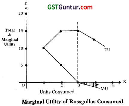
The law describes that, as the consumer has more and more of a commodity, the additional utility which he derives from an additional unit of commodity goes on falling. Marshall stated the law as follows –
“The additional benefit which a person derives from a given increase in stock of a thing diminishes with every increase in the stock that he already has.” The law can be explained with the help of following table:
Table : Utility Schedule

Units of Rossgulla’s Consumed	Total Utility	Marginal Utility
1	TU = U₁ + U₂ + ….. U_n	MU = TU_n – TU_n-1
2	10	10
3	15	5
4	15	0

The above table shows that as the consumer goes on consuming rossgullas, the additional or marginal utility goes on diminishing.
The consumption of 3rd unit of rossgulla gives no additional utility and the 4th unit is giving negative utility.
The 4th unit instead of giving satisfaction causes dissatisfaction.
Total utility goes on increasing as long as MU is positive, but at diminishing rate.
When total utility is highest, marginal utility is zero. This is the point of full satisfaction.
When marginal utility becomes negative, total utility starts falling.
MU is the rate of change in TU or slope of TU curve.
MU can be positive, zero or negative.
We can show the information given in the table on a graph as follows:

The figure shows that marginal utility curve goes on declining as the consumption increases. It even crosses the X-axis and suggest negative marginal utility. Total utility curve rises upto a point and then starts falling.

The Law of Diminishing Marginal Utility helps us to understand how a consumer reaches equilibrium in One Commodity Case:
→ A consumer tries to equalize marginal utility of a commodity with its price in order to maximize the satisfaction. A consumer thus compares the price with the marginal utility of a commodity.

→ He keep on purchasing a commodity till MU > P. In other words, so long as price is less, he buys more which is also the basis of the law of demand.

→ The consumer is at equilibrium where:
Marginal Utility of the commodity = Price of the commodity
MU_x = P_x. MU money
\(\frac{M U_{x}}{P_{x}}\) = MU money

In reality, a consumer spends his money income to buy different commodities. In case of many commodities, consumer equilibrium is explained with the Law of Equi-Marginal Utility:
1. The law states that a consumer will allocate his expenditure in a way that the utility gained from the last rupee spent on each commodity is equal or the marginal utility each commodity is proportional to its price.

2. The consumer is said to be equilibrium when the following condition is met –
\(\frac{M U_{x}}{P_{x}}=\frac{M U_{y}}{P_{y}} M U_{\text {money }}\)
OR
\(\frac{M U_{x}}{M U_{y}}=\frac{P_{x}}{P_{y}}\)
The Law of Diminishing Marginal Utility is based on the following assumptions:
1. Homogeneous Units:

It is assumed that all the units of the commodity are homogeneous ie. identical in every respect like size, taste, colour, quality, blend, etc.
Example – If a consumer is consuming Cadbury Dairy Milk Chocolate (40 gms.), then all bars of chocolate must be of Dairy Milk Chocolates and not of any other type.

2. Continuous Consumption:
There should not be any time gap or interval between the consumption of one unit and another unit.

3. Rationality:
The consumer is assumed to be rational.

4. Cardinal Measurement:
The utility is measurable and quantifiable.

5. Constancy of Marginal Utility of Money:
The marginal utility of money remain unchanged throughout when the consumer is spending on a commodity.

6. The tastes of consumers should remain constant.

Exceptions to and limitations of the Law of Diminishing Marginal Utility:
In some cases a consumer gets increasing marginal utility with the increase in consumption. Such cases are called as exception which are as follows –
1. Hobbies and Rare Collections: The law does not hold good in case of hobbies and rare collections like reading, collection of stamps, coins, etc. Every additional unit gives more satisfaction i.e. the marginal utility tends to increase.

2. Abnormal Persons: The law does not apply to abnormal persons like misers, drunkards, musicians, drug addicts, etc. who want more and more of the commodity they are in love with.

3. Indivisible Goods: The law cannot be applied in case of indivisible bulky goods like T. V. set, house, scooter, etc. No one purchases more than one unit of such goods at a time.

The limitations of the Law of Diminishing Marginal Utility are as follows –
1. Cardinal Measurement Unrealistic: The law assumes cardinal measurement of utility. This is unrealistic, because, utility being a subjective or psychological phenomenon, cannot be measured numerically. The feeling experienced by a consumer cannot be quantified.

2. Unrealistic Conditions: The law is based on unrealistic assumptions. It is not possible to meet all conditions like homogeneous goods, continuous consumption, rationality, etc. at the same time.

3. Constant Marginal Utility of Money: The law assumes that marginal utility of money remains constant. Therefore, the utility of the commodity depends on its quantity alone. But, the marginal utility of money never remains constant.

4. Inapplicable to Indivisible Goods: The assumptions of the Law of DMU cannot be made applicable to indivisible bulky goods like T. V. Sets, scooter, house, etc. because no one purchases more than one unit of such goods at a time.

5. Single Commodity Model: The Law of DMU is a single commodity model. Marginal utility of each commodity is measured independently. But, a consumer may purchase more than one commodity. Also, utilities of goods such as complementary or substitutes are interdependent.

Consumer’s surplus:
Consumers Surplus is one of the important concept in economic theory and in economic policy making. It was given by Dr. Alfred Marshall. Marshall’s concept of consumer surplus is based on the following assumptions:

Utility can be cardinally measured in monetary units.
Marginal utility of money remains constant.
Income, fashion and taste of consumer remains constant.
Independent marginal utility of each unit of the commodity.
The law of diminishing marginal utility holds good.

Explanation:
→ In our daily expenditure, we often find that the price we pay for a commodity is less than the satisfaction derived from its consumption.

→ Therefore, we are ready to pay much higher price for a commodity than we actually have to pay.
Example: Commodities like salt, newspaper, match box, etc. are very useful, but they are also very cheap.

→ From the purchase of such commodities we derive a good deal of extra satisfaction or surplus over and above the price that we pay for them. This is consumer’s surplus.

→ Marshall defined consumer surplus “as the excess of the price which a person would be willing to pay rather than go without the thing over that which he actually does pay”.

→ Thus, it is the difference between what a consumer is ready to pay and what he actually pays.
Consumer Surplus = What a consumer is ready to pay – What he actually pays
= Sum of Marginal Utilities – (Price X Units Purchased)
= Total Utility – Total amount spent.
We can illustrate the concept of consumer’s surplus with the help of following table
Table : Measurement of Consumer’s Surplus

No. of units	Marginal Utility (₹)	Price (₹)	Consumers Surplus
1	25	10	15
2	20	10	10
3	15	10	05
4	10	10	00
Total Units purchased	Total Utility = 70	Total Amt. Spent = 40	30

When the consumer buy first unit of commodity he is ready to pay ₹ 25 for it as he expects satis-faction worth ₹ 25 from it and thus gets a surplus worth ₹ 15. For second unit he is ready to pay only ₹ 20 for it as he expects lesser satisfaction from it and thus gets surplus worth ₹ 10 only. The consumer will go on buying the commodity till Marginal Utility = Price & consumer surplus is Zero Le. upto 4th unit.
Here, Consumer Surplus = Total Utility – Total Amt. Spent = ₹ 70 – ₹ 40 = ₹ 30.
We can represent consumers surplus with the following diagram.

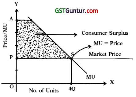
In the diagram MU is the marginal utility curve. OP (Rs. 10) is the market price. In equilibrium, consumer would § buy OQ (4) units (at this MU = P). For OQ (4) units he is required to pay OQ (4 units) X OP (₹ 10) = OQSP(₹ 40). The consumer was ready to pay (by MU curve) OQ SA(₹ 70). Thus, he derives surplus of satisfaction. OQSA(₹ 70) – OQSP(Rs. 40) = PSA(Rs. 30)

The uses/importance of the consumer surplus concept are as follows:
1. Distinction between Value-in-Useand Value-in-exchange: Consumer’s surplus draws a clear distinction between value-in-use and value-in-exchange.
Example – SALT have great value -in-use but much less value-in-exchange. Being necessity and cheap thing, it yield a large consumer surplus. The consumer’s surplus depends on total utility, whereas price depends on marginal utility. The total utility of salt consumed is much greater but its marginal utility (and price) is low due to its excess supply.

2. Comparing Advantages of Different Places: The concept of consumer’s surplus is useful when we compare the advantages of living in two different places. A place with greater amenities available at cheaper rates give large surplus of satisf action to consumers than backward place or region. Consumer’s surplus thus indicates conjunctural advantages, Le. the advantages of environment arid opportunities.

3. To the Businessman and Monopolist: A businessman can raise prices of those goods in which there is a large consumer’s surplus. The seller will be able raise price especially if he is a monopolist and controls the supply of the commodity.

4. Useful to the government in determining taxes: The concept is very useful to Finance Minister in imposing taxes on various goods and fixing their rates. He will tax those goods in which the consumers enjoy large surplus. The consumers thus will have to pay more and their consumer’s surplus will fall.

But at the same time it will raise the revenue of the government. The loss of consumers must be compared with the gains to the government. If the loss of consumers is greater than the gains to government, then, the tax is not proper and vice versa.

5. Measuring Benefits from International Trade: Through international trade, a country can import goods cheaply i.e. a country can get goods at lower price than they are prepared to pay for them. The imports, therefore give larger surplus of satisfaction to people. The larger this surplus, the more beneficial is the international trade.

6. Useful in cost-benefits analysis of projects: While undertaking any project the government usually compare the cost of project and flow of benefits from project both in economic and in non-economic terms.
Example – For Flyover Bridge Project the government will consider the consumers surplus Le. benefits in terms of time saving, fuel saving, etc. expected from flyover bridge project.

The CRITICISMS of the consumer’s surplus concept are as follows:
1. Imaginary: The concept of consumer’s surplus is quite imaginary idea. One has to imagine what you are prepared to pay and you proceed to deduct from that what you actually pay. It is all hypothetical and unreal.

2. Cardinal measurement is not possible: Consumer’s surplus cannot be measured precisely because it is difficult to measure the total utilities and marginal utilities of the commodities consumed in quantitative terms.

3. Ignores the interdependence between goods: The concept of consumer’s surplus does not consider the effect of availability and non-availability of substitutes and complementary goods on the consumption of a particular commodity. Actually consumer surplus derived from a commodity is affected by substitutes and complementary goods.

4. Cannot be measured in terms of money: This is because the marginal utility of money changes as purchases are made and the consumer’s stock of money diminishes. But, Marshall assumed that-the marginal utility of money to be constant.

5. Not applicable to Necessaries: It does not apply to the necessaries of life. In such cases the surplus is immeasurable example – Food and Water. Consumer surplus is infinite because a consumer will stake whole of his income rather than go without them.

6. Not applicable to prestige: example – Diamonds jewellery, etc. fall in their prices lead to a fall in consumer’s surplus.

Indifference Curve Analysis:

An indifference curve is a curve which represents combinations of two commodities that gives same level of satisfaction to the consumer.
As all the combinations give same level of satisfaction, the consumer becomes indifferent (Le. neutral) as to which combination he gets.
In other words, all the combinations lying on indifference curve are equally desirable and equally preferred by the consumer.
To Understand consider the following indifference schedule.

Table : Indifference Schedule:

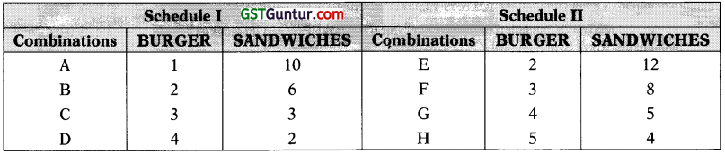
In the schedule I above, the consumer is indifferent whether he gets combination A, B, C or D. This is because all combinations give him same amount of satisfaction and therefore equally preferable to him. He gets as much satisfaction from 1 burger and 10 sandwiches as from 3 burgers and 3 sandwiches.

By plotting the above combinations on a graph, we can derive an indifference curve as shown in the following figure:

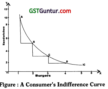
→ In the diagram, quantity of burger is measured on X-axis and quantity of sandwiches on Y-axis. The various combinations A, B, C, D are plotted and on joining them, we get a curve known as indifference curve. All combinations lying on the indifference curve give the same level of satisfaction to the consumer. Hence, the consumer is indifferent among them.

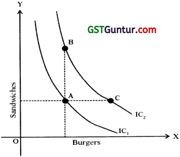
→ If the indifference schedule II is also plotted on the graph, we will get IC₂. This will lie above the IC₁ as all of IC₂ combinations contain greater quantities of burgers and sandwiches. Similarly, we can draw IC₃, IC₄, etc… to make a complete indifference map as follows. Indifference map represents a full description of con¬sumer’s tastes and preferences.

→ In the diagram, the various combinations E, F, G, H on IC₂ give consumer same level of satisfaction and hence equally preferable to the consumer. The consumer is indifferent whether he gets combination E or F or any other combination.

→ The consumer however will prefer any combination lying on IC₂ as it will give him more satisfaction than any combination lying on IC₁

→ This is because combinations lying on IC₂ have larger quantity of burgers and sandwiches.

→ Thus, a higher indifference curve represents a higher level of satisfaction than lower indifference curve but How Much Higher cannot be indicated.

→ It is so because IC system is based on Ordinal Approach according to which utility cannot be quantified but can only be compared.

Assumptions of indifference curve:
Non-satiety: This assumption means that the consumer has not reached the point of full satisfaction in the consumption of any commodity. Therefore, a larger quantity of both com-modities are preferred by the consumer. Larger the quantities of commodities, higher would be the total utility.

Rationality: Consumer is assumed to be rational. He aims at the maximisation of his total utility, given the market prices and money income. He is also assumed to have all relevant information like prices of goods, the markets where they are available, etc.

Consistency: The consumer is consistent in his choice Le. the preferences of consumers are consistent. If he prefers combination ‘A’ over combination ‘B’ in one period of time he will NOT prefer ‘B’ over ‘A’ in another period of time.

Transitivity: If combination A is preferred to B and ‘B’ is preferred to C, then, A is preferred to C. Symbolically, if A>B, and B>C, then A>C.

Ordinal Utility: It is assumed that consumer cannot measure precisely utility or satisfaction in absolute units Le. cardinally, but he can express utility ordinally. In other words, consumer is capable of comparing and ranking satisfaction derived from various goods and their combinations.

Diminishing Marginal Rate of Substitution: It means that as more and more units of ‘A’ are substituted for ‘B’ consumer will sacrifice lesser and lesser units of ‘B’ for each additional unit of ‘A’.

Marginal Rate of Substitution:
→ The concept of marginal rate of substitution is the basis of Indifference Curves in the Theory of Consumer’s Behaviour.

→ It may be defined as the rate at which a consumer will exchange successive units of one good (commodity) for another.

→ Consider the following schedule.
Table: Indifference Schedule:

Combinations	Good X	Good Y	Marginal Rate of Substition = \(\frac { ∆ Y }{ ∆ X }\)
A B C D	1 2 3 4	10 6 4 3	4X : 1X 2Y : 1X 1Y : 1X

→ The above schedule shows the combinations of two goods ‘X’ and ‘Y’. Suppose the consumer wants more of ‘X’. To do so he must sacrifice some units of ‘Y’. in order to maintain same level of satisfaction.

→ Initially, the consumer sacrifices 4Y to get IX, to obtain second unit of ‘X’ he sacrifices 2Y and so on.

→ This rate of sacrifice is technically called Marginal Rate of Substitution (MRS).

→ Thus, for any goods X and Y, the MRS is the loss of Y which can just be compensated by a gain of X. MRSxy goes on diminishing.

→ We can also measure MRS on an indifference curve. Consider the following diagram.

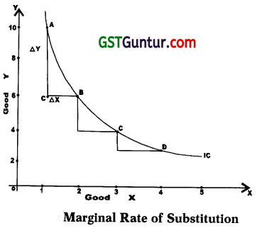
→ In the diagram, when the consumer moves from combination A to combination B, he gives up AC of Y and takes up CB of X and gets the same level of satisfaction.

→ Thus, MRS_XY = \(\frac { AC }{ CB }\) = \(\frac { ∆Y }{ ∆X }\) and so on.

→ MRS_XY between two points is also the slope of the indifference curve between these two points. As the consumer moves from combination B to C, C to D, the MRS_XY goes on diminishing.

The MRS goes on diminishing due to following reasons –
1. The want for a particular commodity is satiable. So, as the consumer has more and more of that commodity, he is willing to take less and less of it. Thus, in the above example, when the consumer has more and more of ‘X’, his intensity of want for X’ diminishes but for ‘Y’ increases. Therefore, he does not want more of ‘X’ now and is not ready to H sacrifice more number of ‘Y’ for ‘X’.

2. The second reason is that, the goods are not perfect substitutes of each other in the satisfaction of particular want. If they are perfect substitutes, the MRS would not fall and remain constant.

Indifference curves always slope downwards from left to right:

This means that an indifference curve has a negative slope.
REASON – In order to maintain same level of satisfaction, as the quantity of burgers is increased in the combination, the quantity of sandwiches is reduced.
Thus, this property follows from the definition of an IC and non-satiety assumption i.e. more is preferred to less.
Indifference curve cannot be horizontal straight line or vertical straight line or positively sloped.

Indifference Curves are convex to the origin:

This means that IC is relatively steeper first in its left hand portion and tends to become relatively flatter in its right hand portion.
REASON: Diminishing Marginal Rate of Substitution.
The schedule and diagram shows that the consumer sacrifices less and less of sandwiches for every additional unit of burger.
The convexity of an IC means that the two commodities can substitute each other but are not perfect substitute.
If IC were concave to origin, it would mean increasing MRS. This is against the assumption of diminishing MRS.
Similarly, IC cannot be straight lines as it would mean that MRS remains constant (for perfect substitute.)

Higher Indifference Curves Represents Higher Level of Satisfaction:
1. In an indifference map, combinations lying on a higher IC gives higher level of satis-faction than the combinations lying on a lower IC. But how much higher cannot be indicated.

2. REASON: This is because combinations on higher IC contains more quantity of either sandwiches or burger without having less of other as shown in the following diagram.

3. Combinations B and C on IC₂ will be preferred by the consumer than the combination A on IC₁.

4. Combination B on IC₂ contains more quantity of sandwiches without having less of burgers compared to combination A on IC₁.

5. Hence, all combinations on IC₂ gives more satisfaction to consumer. Thus, higher IC represents higher satisfaction.

Indifference curves cannot intersect each other:
1. It means that only one IC will pass through a point in the indifference map.

2. In other words, ONE combination can lie only on one IC.

3. Higher IC represents higher level of satisfaction and lower IC represents lower level of satisfaction. If they intersect each other, it would lead to illogical result.

4. It can be proved with the help of following diagram –

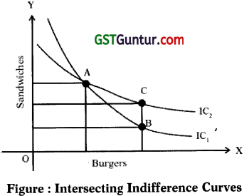
In the diagram two IC intersect each other at point A. On IC₁; combinations A = B and on IC₂, Combinations A = C. Therefore, by assumption of transitivity if, A = B and A = C ∴ B = C. But C > B as it lie on higher IC giving higher satisfaction due to more quantity of sandwiches. So two IC cannot intersect.

Indifference curve will not touch either X-axis or Y-axis:
1. The indifference curve will not touch either X-axis or Y-axis because we have assumed that consumer is considering the different combinations of TWO commodities.

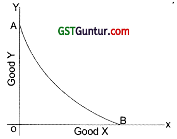
2. If IC touches either of the axis, it would mean that consumer is interested in one commodity only.

3. In the diagram IC touches X-axis at point B and Y-axis at point A.

4. At point B the consumer is satisfied with OB quantity of X-commodity and zero quantity of A. Thft is against the definition of IC. Therefore, IC curve will not touch either axis.

Budget Line Or Price Line (Or Price Opportunity Line Or Expenditure Line Or Budget Constraint or Consumption Possibility Line):
→ A higher indifference curve shows a higher level of satisfaction than lower one.

→ Therefore, to maximize satisfaction consumer will try to reach the highest possible indifference curve.

→ He will try to buy more and more goods to get more and more satisfaction. But, what and how much a consumer can actually buy depends on –

The money income of consumer.
Prices of goods he wants to buy. They are the two objective factors which form the ® budgetary constraint of the consumer.

The budgetary position of the consumer can be graphically shown by BUDGET LINE. A budget line or price line shows maximum quantity of the different combinations of TWO GOODS that the consumer can purchase with his given money income and given market prices of goods.
Example:
The consumer’s money income is ₹ 100 to spend on X and Y.
Price of X is ₹ 5 per unit
Price of Y is ₹ 2 per unit
Therefore, the consumer can get either 20 units of X and no Y.
OR
50 units of Y and no X.
OR
Combination of X and Y
Hence, 20 X and 50 Y form the two extreme limits of his expenditure. But the consumer can buy any ONE of the many combinations of X and Y within these limits. Graphically it can be shown as follows –

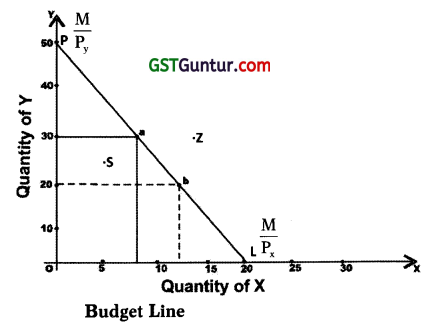
→ This budget line corresponds to the following equation, called Budget Line Equation
P_x. X + P_y. Y = M
Where –
M = Total Money Income
P_x = Price of commodity ‘X’
X = Quantity of X commodity
P_y = Price of commodity
Y = Quantity of Y’ commodity

→ It can be seen in the diagram that the consumer can buy a maximum of 20 units of X as denoted by points ‘L’ or buy a maximum of 50 units of Y as denoted by point On joining points P &L, we get a line PL called as budget line. It determines the limit or boundary of purchase.

→ The consumer can choose any combination of X and Y lying on budget line like combinations ‘a’ (8 X & 30 Y) or ‘b’ (12 X & 20 Y) or any other combination. However, the consumer cannot choose combination ‘Z’ as it is beyond his means Le. budget. Any combination like ‘S’ lying within the budget line, shows under spending by consumer.

→ The slope of budget line is equal to the ratio of the prices of two goods Le. ratio of the prices of X to the price of Y. Thus, the slope of the budget line PL is \(\frac { Px }{ Py }\)

Consumer’s equilibrium:
→ The consumer is said to be in equilibrium when he maximizes his satisfaction (Le. utility).

→ To explain the consumer’s equilibrium under ordinal approach, we have to make use of Two tools of indifference curve analysis namely-

the consumer’s Indifference Map, and
his Price/budget line.

Assumptions:

The consumer has a fixed amount of money income to spend.
The consumer intends to buy Two goods.
The Consumer is Rational and tries to maximise his satisfaction.
The prices of two goods are Given and are Constant. Therefore, budget line has constant slope.
Goods are Homogeneous and divisible.
The scale of preference of consumer Le. his taste & preferences remains unchanged. Scale of preference is expressed through indifference map.

→ The Consumer’s Indifference Map shows all indifference curves which rank the consumer’s preferences between various possible combinations of TWO commodities.

→ To maximises his satisfaction consumer would like to reach highest possible indifference curve.

→ The slope of IC at any one point shows the Marginal rate of Substitution (which diminishes).

→ Thus, MRS_xy = \(\frac{M U_{x}}{M U_{y}}\)

→ To maximise satisfaction consumer will try to reach the highest possible IC and so will try to buy more and more of the two commodities.

→ But there are limits to which he can go on and on.

→ These limits are imposed –

his money income, &
prices of the commodities.

→ These limits are described by PRICE/BUDGET LINE which shows the various combinations of two commodities the consumer can afford to buy.

→ All the combinations lying on the budget line are affordable by the consumer. Any, combination lying beyond budget line is unaffordable.

→ The slope of budget/price line shows the ratio of the prices of two commodities i.e.

→ Now we can show how a consumer reaches equilibrium i.e, how he allocates his money expenditure between commodities X and Y and gets maximum satisfaction.

→ For showing this, we will have to superimpose the price line on the indifference map as follows –

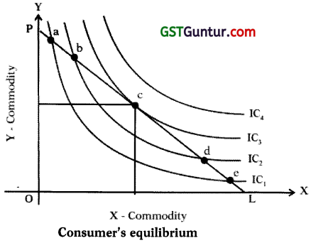
→ In order to maximise his satisfaction, the consumer will try to reach highest IC ie. IC₄.

→ But the budget constraint forces him to remain On the budget line.

→ In the diagram, budget line PL shows all the combinations of X & Y that the consumer can buy. In diagram, we find combinations a, b, c, d, e lie on budget line PL and hence are affordable.

→ Points a,b,d and e lie on lower ICs and so are not the points of equilibrium as the consumer can get more satisfaction with the same amount of money.

→ Point ‘C’is the point of equilibrium as it lies on budget line and also on highest possible indifference curve IC₃ giving maximum satisfaction.

→ At ‘point’ ‘C’, the budget line PL is TANGENT to indifference curve IC₃.

→ At the point of tangency, Slope of indifference Curve = Slope of Budget Line
MRS_XY = \(\frac { Px }{ Py }\)

→ Thus, the consumer is at equilibrium when –

MRS_XY = \(\frac { Px }{ Py }\) and
Indifference curve is CONVEX to origin.

Supply

Meaning:
Supply of a commodity refers to the quantity of commodity offered for sale at a particular price [ during a given period of time. Thus, the supply of a commodity may be defined as the amount of commodity which the sellers or producers are able and willing to offer for sale at a particular price, during a given period of time.

Thus, defined, the term supply shows the following features:
1. Supply of a commodity is always with reference to a Price.

2. Supply of a commodity is to be referred to In a given period of time.

3. Supply of a commodity depends on the Ability of seller to supply a commodity However, ability of a seller to supply a commodity depends ON THE STOCK available with him.

4. Supply of a commodity also depends on the Willingness of seller to supply a i commodity. A seller’s willingness to supply a commodity depends On the difference between the reservation price and the prevailing market price.
Example : A dairy farm’s daily supply of milk at the price of ₹ 12 per litre is 600 litres

Determinants of Supply:
Supply of a commodity depends on many factors like price of the commodity, price of related goods, prices of factors of production, technology, etc. All determinants of supply can be expressed in the form of supply function as follows-
S_x = f(P_x, P_y, P_f, T, O……….. )
Where – S_x = Quantity supplied of commodity x
f = function of (depends on)
Px = Price of commodity x
Pr = Price of related commodities
Pf = Prices of factors of production.
T = Technology
O = Objectives/Goals of the firm

Price of the commodity :

Other things being equal the supply of a commodity is DIRECTLY related with its price.
It means that, larger quantity of a commodity is offered for sale at higher price and vice versa.
This is because the profits of the firm increases if the price of its product increases.

Price of the related commodities :

The supply of a commodity also depends on the prices of related commodities i.e. sub-stitute goods and complementary goods.
Other things being equal, if the price of a substitute goes up, the firms will be tempted to produce that substitute to get higher profits. Example – If the price of coffee rises, the firm would reduce the quantity supplied of tea.
On the other hand, other things being equal/if price of a complementary good goes up, the supply of the product in question also rises. Example – If the prices of fountain pens rise, it may cause an increase in the supply of ink.

Prices of factors of production :

Supply of a commodity depends on the cost of production. The cost of production itself depends upon the prices of various factors of production.
So, if the price of any factor of production rises, the production costs would be higher for the same level of output (and vice versa), Hence the supply will tend to decrease.
Conversely, a fall in the cost of production tends to increase the supply.

State of technology :

A change in technology affects the supply of commodity.
A technological progress and improvement in the methods of production increases productivity, reduce the cost of production and increases the profits. As a result more is produced and supplied.
Also discoveries and innovations bring new variety of goods.

Objectives of the firm :

The objectives of the firm and business policy pursued by it also affect the supply of the product produced by it.
Some firms believes in higher margin of profits and lower turnover while others believe in lower margin of profit and higher turnover (Le. sales) to capture the market or to improve status, goodwill and prestige in the market.

Government Policy:

The supply of a commodity is also affected by the economic policies followed by the Government.
The Government may impose taxes on commodities in the form of excise duty, sales tax and import duties or may give subsidies.
Any increase in such taxes will raise the cost of production and so the quantity supplied will fall. Under such conditions supply will increase only when its price in the market rises.
Subsidies reduce the cost of production and thus encourages firms to produce and sell more.

Time:

Supply is a function of time also.
In a short period, it is not possible to adjust supply to the conditions of demand.
If the time period is sufficiently long, all possible adjustments can be made in the production apparatus and the supply can be fully adjusted to demand.

Number of firms :
1. If the number of firms producing a product increases, the market supply of the product will also increase and vice-versa.

Other factors :
1. Supply of a commodity also depends upon Natural conditions like rainfall, temperature, etc.; industrial and foreign policies, infrastructural facilities; War; market structure; etc.

Law of Supply:
→ Law of Supply express the nature of functional relationship between the price of a commodity and its quantity supplied.

→ It simply states that supply varies DIRECTLY to the changes in price Le. supply of a commodity expands when price rises and contracts when price falls.

→ “The Law of Supply states that the higher the price, the greater the quantity supplied or the lower the price the smaller the quantity supplied, other things remaining the same.” (Dooley)

→ Thus, there is DIRECT RELATIONSHIP between supply and price.

→ It is assumed that other determinants of supply are constant and Only price is the variable and influencing factor. Thus, the law of supply is based on the following main assumptions:-

Cost of production remains unchanged even though the price of the commodity changes.
The technique of production remains unchanged.
Government policies like taxation policy, trade policy, etc. remains unchanged.
The prices of related goods remains unchanged.
The scale of production remains unchanged etc.

→ The law can be explained with the help of supply schedule and a corresponding supply curve.
Table : Supply Schedule

Price ₹ per unit

Supply per week in units

→ The supply schedule shows that when price rises from ₹ 10 per unit to ₹ 20 per unit, the supply also rises from 20 units per week to 30 units per week and so on.

→ Thus, it shows a direct relationship between price and quantity supplied other things being equal.

→ A supply curve is the supply schedule depicted on the graph. The supply curve shows the same information as the supply schedule.

→ In the diagram, the supply curve is sloping upwards from left to right showing a direct relationship between the price and quantity supplied.

→ A single point on supply curve show a single price-supply relationship Example – Point ‘C’ show that if price is ₹ 30, quantity supplied is 40 units.

→ The law of supply states that, supply of a commodity varies directly with its price.

→ But, in some cases, this may not hold true. Hence, the law of supply has the following Exceptions –
1. When the seller expects a further rise in the prices in future, he may hoard stock of commodity. So the supply at present will fall and vice versa.

2. At higher wage rates, there is tendency among labourers to prefer more leisure than work. As a result when wages rise, labour supply falls.

3. In the case of rare commodities like paintings, coins, etc. the supply is fixed. Whatever the price, it cannot change.

4. In an auction or in all those cases where the seller wants to get rid of his goods, he will sell the goods at whatever price they fetch.

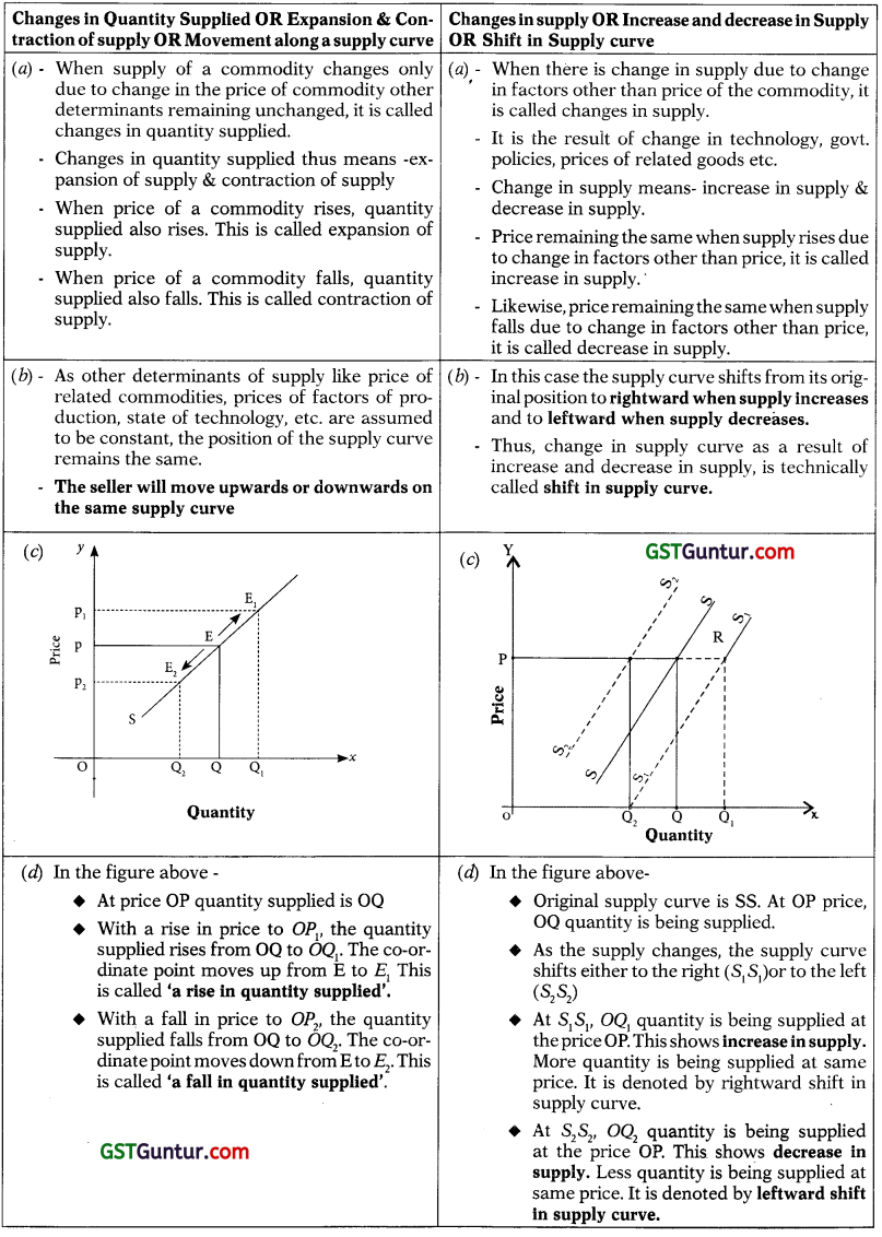
Elasticity of supply:
→ Price elasticity of supply measures the degree of responsiveness of quantity supplied of a commodity to a change in its own price.

→ In other words, the elasticity of supply shows the degree of change in the quantity supplied in response to change in the price of the commodity.

→ Elasticity of supply can be defined “as a ratio of the percentage change in the quantity supplied of a commodity to the percentage change in its own price”.

→ It may be expressed as follows –

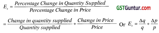
Where – Es = Elasticity of supply
Q = Original quantity supplied
P = Original price
∆ = indicates change
Rearranging the above expression we get – Es = \(\frac{\Delta q}{q} \times \frac{p}{\Delta p}=\frac{\Delta q}{\Delta p} \times \frac{p}{q}\)
→ Since the law of supply establishes positive relationship between price and quantity supplied, the elasticity of supply would be positive.

→ However, in case of decreasing cost industry elasticity of supply is negative.

→ The value of elasticity co-efficient will vary from zero to infinity.

→ The elasticity of supply, according to its degree, may be of following types:
1. Perfectly Inelastic Supply: E_s = 0:
When a change in the price of a commodity has no effect on its quantity supplied, then supply is perfectly inelastic. Example – If price rises by 20% and the quantity supplied remains unchanged then E_s = \(\frac { 0 }{ 20 }\) = 0. In this case, the supply curve is a vertical straight line curve parallel to Y-axis as shown in the figure.

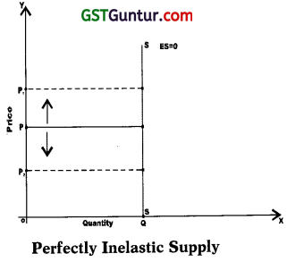
The figure shows that, whatever the price quantity supplied of the com-modity remains unchanged at OQ.

2. Perfectly Elastic Supply: (E_s = ∞):
When with no change in price or with very little change in price, the supply of a commodity expands or contracts to any extent, the supply is said to be perfectly elastic. In this case, the supply is a horizontal straight line and parallel to X-axis

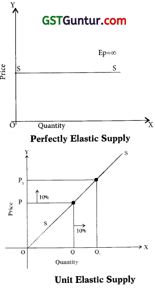
The figure shows (E_s = ∞) that, at given price supply is ever increasing.

3. Unit Elastic Supply : (E_s = 1):
When the percentage change in price is equal to percentage change in quantity supplied, then the supply is said to be unit elastic.
Example – If price rises by 10% and the supply also rises by 10% then, Es = \(\frac { 10 }{ 10 }\) = 1
In this case the straight line supply- curve SS when extended will pass through origin.

4. Relatively/More Elastic Supply: (E_s > 1):
When a small change in price leads to big change in quantity supplied, then the supply is said to be relatively or more elastic.
Example – If price rises by 10% and supply rises by 30% then, 30 E_s = \(\frac { 30 }{ 10 }\) = 3 > 1. The coefficient of elasticity would be somewhere between One and s 10 Infinity. The elastic supply curve is flatter as shown below-

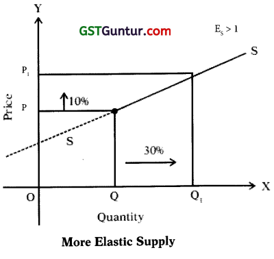
Supply curve SS is flat suggesting that the supply is more elastic. In this case the supply curve SS when extended will pass through Y-axis.

5. Relatively Inelastic Or Less Elastic Supply: (E_s(1):
When a big change in price leads to small change in quantity supplied, then supply is said to relatively inelastic or less elastic.
Example – If price rises by 30% and supply rises by 10% then, E_s = \(\frac { 10 }{ 30 }\) = \(\frac { 1 }{ 3 }\)(1. The coefficient of elasticity would be somewhere between ZERO and ONE. The supply curve in this case has steep slope as shown below –
Supply curve SS is steeply sloped suggesting that supply is less elastic. In this case the supply curve SS when extended will pass through X-axis.

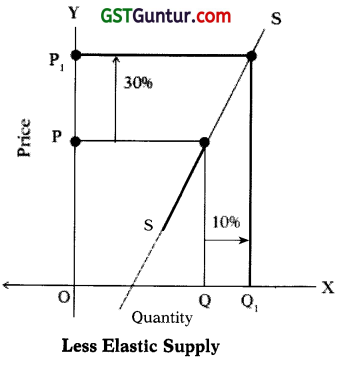
Measurement of Elasticity of Supply:
The different methods of measuring price elasticity of supply are:

The Percentage or Ratio or Proportional Method,
The Point or Geometric Method, and
The Arc Method

1. The Percentage Method:
Thus method is based on the definition of elasticity of supply. The coefficient of price elas-ticity of supply is measured by taking ratio of percentage change in supply to the percentage change in price. Thus, we measure the elasticity by using the following formula

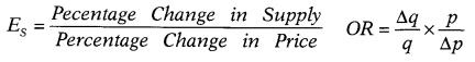
If the coefficient of above ratio is equal to One, the supply will be unitary.
If the coefficient of above ratio is More than one, the supply is relatively elastic.
If the coefficient of above ratio is Less than one, the supply is relatively inelastic.

2. The Point Or Geometric Method:
In point elasticity method, we measure elasticity at a given point on a supply curve.
We can measure E at point ‘R’ in the following manner
i. Extend the supply curve ‘S’ towards the extension of X-axis so that it cuts X-axis at T.
ii. Draw a perpendicular from ‘R’ cutting X-axis at ‘M’
iii. Take the ratio of intercepts MT and OM.
E_s = \(\frac { MT }{ OM }\)
In the figure MT > OM, elasticity is Greater than one.

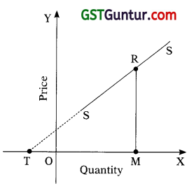
In the adjoining figure, supply curve when extended meets X-axis to the right of the point of origin so that E_s = \(\frac { MT }{ OM }\) ie. MT < OM and so elasticity is Less than unity

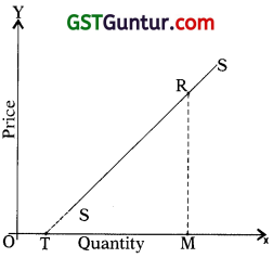
In the adjoining figure, supply curve when extended meets X-axis exactly at the point of origin so that E_s = \(\frac { MT }{ OM }\) = 1, ie. MT = OM and so elasticity of supply is Equal to unity/one.

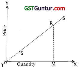
3. The Arc Elasticity Method:
Under this method we measure elasticity of supply over an ARC of the supply curve. The arc elasticity is a measured of the “average elasticity” i.e. elasticity at MID-POINT that connects the two points on the supply curve. Thus, an arc is a portion of a curved line, hence a portion of supply curve. The formula used is –

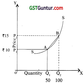
E_s = \(\frac{q_{1}-q_{2}}{q_{1}+q_{2}} \times \frac{p_{1}+p_{2}}{p_{1}-p_{2}}\)
Where – P₁ & q₁ = Original price and quantity
P₂ & q₂ = New price and quantity.
E_s = \(\frac{50-100}{50+100} \times \frac{10+15}{10-15}\)
= E_s = \(\frac{-50}{150} \times \frac{25}{-5}\)
= + 1.66

Equilibrium Price:
1. Equilibrium means a market situation where the quantity demanded is equal to quantity supplied. Thus, the two factors determining equilibrium price are market demand and market supply.

2. Equilibrium price is the price at which the sellers of a good are willing to sell the quantity which buyers want to buy. Thus, equilibrium price (also called market clearing price) is the price at which demand and supply are equal.

3. At equilibrium price both sellers and buyers are satisfied.

4. At equilibrium price, there is neither SHORTAGE nor SURPLUS. So at equilibrium price, market is said to be CLEARED.

5. The following table and figure explains the equilibrium price.

Price of Good-X (₹)	Quantity Demanded of Good-X (units)	Quantity Supplied of Good-X (units)	Effect on Price
5	100	500	Downward
4	200	400	Downward
3	300	300	Equilibrium
2	400	200	Upward
1	500	100	Upward

6. Equilibrium is struck a point E where the demand and supply curve intersect each other.

7. At E, equilibrium price is OP i.e. ₹ 3 and equilibrium quantity is OQ i.e. 300 units.

8. When the price is ₹ 5 per unit, the quantity demanded is 100 units and quantity supplies is 500 units. It is situation where market demand < market supply and there is excess supply i.e., surplus supply. At a given price, sellers are willing to sell more than what buyers are ready to buy. As a result of pressure of excess supply the market price falls to ₹ 4.

9. At a price of ₹ 4. the pressure of excess supply still continues and hence the price falls further to ₹ 3.

10. At a price of ₹ 3, the market is Cleared as the quantity demanded and supplied are equal to each other. There, is no Surplus.

11. Thus, we can conclude that pressure of excess supply (surplus) reduces the price.

12. Similarly, if the price is ₹ 1, the quantity demanded is 500 units and quantity supplied is 100 units. It is a situation where market demand market supply and there is excess demand or Shortage of supply. As a result of excess demand or SHORTAGE of supply the market price will rise. So long as pressure of excess demand continues price will rise i.e. till point E. At point E, excess demand is eliminated and quantity demand and supplied are equal to each other. The market has Cleared.

13. Thus, we can conclude that pressure of excess demand (shortage of supply) increases the price.

14. The equilibrium price is determined by the intersection between demand and supply therefore, it is also called as the Market equilibrium.

Theory of Demand and Supply – Business Economics CA Foundation Notes Chapter 2

Leave a Comment Cancel Reply